Introduction
- this is a book on STARKs
- it is a work in progress
Finite Fields
Functions and low-degree extension
Extension Fields
Code Theory
- I think “succinct proofs and linear algebra” provides a good intro and notation
Hamming weight
hamming weight of a string is the number of non-zero entries.
The Hamming weight of a string is the number of symbols that are different from the zero-symbol of the alphabet used
For we have:
\text{hamming_weight}(s) = 3
in other words for we have:
\text{hamming_weight}(\vec{x}) = |{ i | x[i] \neq 0 }|
Hamming Distance
In information theory, the Hamming distance between two strings of equal length is the number of positions at which the corresponding symbols are different.
\text{hamming_distance}(\vec{x}, \vec{y}) = |{ i | x[i] \neq y[i] }|
Repeated code
( is the identity, repeated times in the matrix)
( repeated times)
Reed–Solomon error correcting code
“the RS code of rate evaluated over ”.
Johnson bound
What is Johnson bound?
TODO: We should explain it here, and also make sure we have defined everything we need to understand it.
Let be a code with minimum relative distance , for . Then is -list-decodable for every .
TODO: is this the conjecture, or is conjecture 2.3 from the DEEP paper the conjecture based on the Jonhson bound?
AIR
- check https://cronokirby.com/posts/2022/09/notes-on-stark-arithmetization/
Overview
Here’s some notes on how STARK works, following my read of the ethSTARK Documentation (thanks Bobbin for the pointer!).
Warning: the following explanation should look surprisingly close to PlonK or SNARKs in general, to anyone familiar with these other schemes. If you know PlonK, maybe you can think of STARKs as turboplonk without preprocessing and without copy constraints/permutation. Just turboplonk with a single custom gate that updates the next row, also the commitment scheme makes everything complicated.
The execution trace table
Imagine a table with columns representing registers, which can be used as temporary values in our program/circuit. The table has rows, which represent the temporary values of each of these registers in each “step” of the program/circuit.
For example, a table of 3 registers and 3 steps:
| r0 | r1 | r2 | |
|---|---|---|---|
| 1 | 0 | 1 | 534 |
| 2 | 4 | 1 | 235 |
| 3 | 3 | 4 | 5 |
The constraints
There are two types of constraints which we want to enforce on this execution trace table to simulate our program:
- boundary constraints: if I understand correctly this is for initializing the inputs of your program in the first rows of the table (e.g. the second register must be set to 1 initially) as well as the outputs (e.g. the registers in the last two rows must contain , , and ).
- state transitions: these are constraints that apply to ALL contiguous pairs of rows (e.g. the first two registers added together in a row equal the value of the third register in the next row). The particularity of STARKs (and what makes them “scallable” and fast in practice) is that the same constraint is applied repeatidly. This is also why people like to use STARKs to implement zkVMs, as VMs do the same thing over and over.
This way of encoding a circuit as constraints is called AIR (for Algebraic Intermediate Representation).
Straw man 1: Doing things in the clear coz YOLO
Let’s see an example of how a STARK could work as a naive interactive protocol between a prover and verifier:
- the prover constructs the execution trace table and sends it to the verifier
- the verifier checks the constraints on the execution trace table by themselves
This protocol works if we don’t care about zero-knowledge, but it is obviously not very efficient: the prover sends a huge table to the verifier, and the verifier has to check that the table makes sense (vis a vis of the constraints) by checking every rows involved in the boundary constraints, and checking every contiguous pair of rows involved in the state transition constraints.
Straw man 2: Encoding things as polynomials for future profit
Let’s try to improve on the previous protocol by using polynomials. This step will not immediately improve anything, but will set the stage for the step afterwards. Before we talk about the change to the protocol let’s see two different observations:
First, let’s note that one can encode a list of values as a polynomial by applying a low-degree extension (LDE). That is, if your list of values look like this: , then interpolate these values into a polynomial such that
Usually, as we’re acting in a field, a subgroup of large-enough size is chosen in place of as domain. You can read why’s that here. (This domain is called the “trace evaluation domain” by ethSTARK.)
Second, let’s see how to represent a constraint like “the first two registers added together in a row equal the value of the third register in the next row” as a polynomial. If the three registers in our examples are encoded as the polynomials then we need a way to encode “the next row”. If our domain is simply then the next row for a polynomial is simply . Similarly, if we’re using a subgroup generated by as domain, we can write the next row as . So the previous example constraint can be written as the constraint polynomial .
If a constraint polynomial is correctly satisfied by a given execution trace, then it should be zero on the entire domain (for state transition constraints) or on some values of the domain (for boundary constraints). This means we can write it as for some “quotient” polynomial and the evaluation points (that encode the rows) where the constraint should apply. (In other words, you can factor using its roots .)
Note: for STARKs to be efficient, you shouldn’t have too many roots. Hence why boundary constraints should be limited to a few rows. But how does it work for state transition constraints that need to be applied to all the rows? The answer is that since we are in a subgroup there’s a very efficient way to compute . You can read more about that in Efficient computation of the vanishing polynomial of the Mina book.
At this point, you should understand that a prover that wants to convince you that a constraint applies to an execution trace table can do so by showing you that exists. The prover can do so by sending the verifier the polynomial and the verifier computes from the register polynomials and verifies that it is indeed equal to multiplied by the . This is what is done both in Plonk and in STARK.
Note: if a constraint doesn’t satisfy the execution trace, then you won’t be able to factor it with as not all of the will be roots. For this reason you’ll get something like for some “rest” polynomial. TODO: at this point can we still get a but it will have a high degree? If not then why do we have to do a low-degree test later?
Now let’s see our modification to the previous protocol:
- Instead of sending the execution trace table, the prover encodes each column of the execution trace table (of height ) as polynomials, and sends the polynomials to the verifier.
- The prover then creates the constraint polynomials (as described above) for each constraint involved in the AIR.
- The prover then computes the associated quotient polynomials (as described above) and sends them to the verifier. Note that the ethSTARK paper call these quotient polynomials the constraint polynomials (sorry for the confusion).
- The verifier now has to check two things:
- low-degree check: that these quotient polynomials are indeed low-degree. This is easy as we’re doing everything in the clear for now (TODO: why do we need to check that though?)
- correctness check: that these quotient polynomials were correctly constructed. For example, the verifier can check that for by computing themselves using the execution trace polynomials and then checking that it equals . That is, assuming that the first constraint only apply to the first row .
Straw man 3: Let’s make use of the polynomials with the Schwartz-Zippel optimization!
The verifier doesn’t actually have to compute and compare large polynomials in the correctness check. Using the Schwartz-Zippel lemma one can check that two polynomials are equal by evaluating both of them at a random value and checking that the evaluations match. This is because Schwartz-Zippel tells us that two polynomials that are equal will be equal on all their evaluations, but if they differ they will differ on most of their evaluations.
So the previous protocol can be modified to:
- The prover sends the columns of the execution trace as polynomials to the verifier.
- The prover produces the quotient polynomials and sends them to the verifier.
- The verifier produces a random evaluation point .
- The verifier checks that each quotient polynomial has been computed correctly. For example, for the first constraint, they evaluate at , then evaluate , then check that both evaluations match.
Straw man 4: Using commitments to hide stuff and reduce proof size!
As the title indicates, we eventually want to use commitments in our scheme so that we can add zero-knowledge (by hiding the polynomials we’re sending) and reduce the proof size (our commitments will be much smaller than what they commit).
The commitments used in STARKs are merkle trees, where the leaves contain evaluations of a polynomial. Unlike the commitments used in SNARKs (like IPA and KZG), merkle trees don’t have an algebraic structure and thus are quite limited in what they allow us to do. Most of the complexity in STARKs come from the commitments. In this section we will not open that pandora box, and assume that the commitments we’re using are normal polynomial commitment schemes which allow us to not only commit to polynomials, but also evaluate them and provide proofs that the evaluations are correct.
Now our protocol looks like this:
- The prover commits to the execution trace columns polynomials, then sends the commitments to the verifier.
- The prover commits to the quotient polynomials, the sends them to the verifier.
- The verifier sends a random value .
- The prover evaluates the execution trace column polynomials at and (remember the verifier might want to evaluate a constraint that looks like this as it also uses the next row) and sends the evaluations to the verifier.
- The prover evaluates the quotient polynomials at and sends the evaluations to the verifier (these evaluations are called “masks” in the paper).
- For each evaluation, the prover also sends evaluation proofs.
- The verifier verifies all evaluation proofs.
- The verifier then checks that each constraint is satisfied, by checking the equation in the clear (using the evaluations provided by the prover).
Straw man 5: a random linear combination to reduce all the checks to a single check
If you’ve been reading STARK papers you’re probably wondering where the heck is the composition polynomial. That final polynomial is simply a way to aggregate a number of checks in order to optimize the protocol.
The idea is that instead of checking a property on a list of polynomials, you can check that property on a random linear combination. For example, instead of checking that and , and , you can check that for random values you have:
Often we avoid generating multiple random values and instead use powers of a single random value, which is a tiny bit less secure but much more practical for a number of reasons I won’t touch here. So things often look like this instead, with a random value :
Now our protocol should look like this:
- The prover commits to the execution trace columns polynomials, then sends the commitments to the verifier.
- The verifier sends a random value .
- The prover produces a random linear combination of the constraint polynomials.
- The prover produces the quotient polynomial for that random linear combination, which ethSTARK calls the composition polynomial.
- The prover commits to the composition polynomial, then sends them to the verifier.
- The protocol continues pretty much like the previous one
Note: in the ethSTARK paper they note that the composition polynomial is likely of higher degree than the polynomials encoding the execution trace columns. (The degree of the composition polynomial is equal to the degree of the highest-degree constraint.) For this reason, there’s some further optimization that split the composition polynomial into several polynomials, but we will avoid talking about it here.
We now have a protocol that looks somewhat clean, which seems contradictory with the level of complexity introduced by the various papers. Let’s fix that in the next blogpost on FRI…
FRI
Cairo
Check cairo book: https://book.cairo-lang.org/
There’s different ways to write for the Cairo VM:
- using Cairo instructions directly, documented in the Cairo paper (good luck)
- using Cairo 0, a low-level language documented here https://docs.cairo-lang.org/how_cairo_works/builtins.html
- using Cairo 1, a rust-like high-level language documented here https://book.cairo-lang.org/
Public Memory
Here are some notes on how the Cairo zkVM encodes its (public) memory in the AIR (arithmetization) of the STARK.
If you’d rather watch a 25min video of the article, here it is:
The AIR arithmetization is limited on how it can handle public inputs and outputs, as it only offer boundary constraints. These boundary constraints can only be used on a few rows, otherwise they’re expensive to compute for the verifier. (A verifier would have to compute for some given , so we want to keep small.)
For this reason Cairo introduce another way to get the program and its public inputs/outputs in: public memory. This public memory is strongly related to the memory vector of cairo which a program can read and write to.
In this article we’ll talk about both. This is to accompany this video and section 9.7 of the Cairo paper.
Cairo’s memory
Cairo’s memory layout is a single vector that is indexed (each rows/entries is assigned to an address starting from 1) and is segmented. For example, the first rows are reserved for the program itself, some other rows are reserved for the program to write and read cells, etc.
Cairo uses a very natural “constraint-led” approach to memory, by making it write-once instead of read-write. That is, all accesses to the same address should yield the same value. Thus, we will check at some point that for an address and a value , there’ll be some constraint that for any two and such that , then .
Accesses are part of the execution trace
At the beginning of our STARK, we saw in How STARKs work if you don’t care about FRI that the prover encodes, commits, and sends the columns of the execution trace to the verifier.
The memory, or memory accesses rather (as we will see), are columns of the execution trace as well.
The first two columns introduced in the paper are called and . For each rows in these columns, they represent the access made to the address in memory, with value . As said previously, we don’t care if that access is a write or a read as the difference between them are blurred (any read for a specific address could be the write).
These columns can be used as part of the Cairo CPU, but they don’t really prevent the prover from lying about the memory accesses:
- First, we haven’t proven that all accesses to the same addresses always return the same value .
- Second, we haven’t proven that the memory contains fixed values in specific addresses. For example, it should contain the program itself in the first cells.
Let’s tackle the first question first, and we will address the second one later.
Another list to help
In order to prove that the two columns in the part of the execution trace, Cairo adds two columns to the execution trace: and . These two columns contain essentially the same things as the columns, except that these times the accesses are sorted by address.
One might wonder at this point, why can’t L1 memory accesses be sorted? Because these accesses represents the actual memory accesses of the program during runtime, and this row by row (or step by step). The program might read the next instruction in some address, then jump and read the next instruction at some other address, etc. We can’t force the accesses to be sorted at this point.
We will have to prove (later) that and represent the same accesses (up to some permutation we don’t care about).
So let’s assume for now that correctly contains the same accesses as but sorted, what can we check on ?
The first thing we want to check is that it is indeed sorted. Or in other words:
- each access is on the same address as previous:
- or on the next address:
For this, Cairo adds a continuity constraint to its AIR:
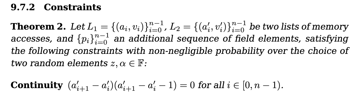
The second thing we want to check is that accesses to the same addresses yield the same values. Now that things are sorted its easy to check this! We just need to check that:
- either the values are the same:
- or the address being accessed was bumped so it’s fine to have different values:
For this, Cairo adds a single-valued constraint to its AIR:

And that’s it! We now have proven that the columns represent correct memory accesses through the whole memory (although we didn’t check that the first access was at address , not sure if Cairo checks that somewhere), and that the accesses are correct.
That is, as long as contains the same list of accesses as .
A multiset check between and
To ensure that two list of elements match, up to some permutation (meaning we don’t care how they were reordered), we can use the same permutation that Plonk uses (except that plonk fixes the permutation).
The check we want to perform is the following:
But we can’t check tuples like that, so let’s get a random value from the verifier and encode tuples as linear combinations:
Now, let’s observe that instead of checking that these two sets match, we can just check that two polynomials have the same roots (where the roots have been encoded to be the elements in our lists):
Which is the same as checking that
Finally, we observe that we can use Schwartz-Zippel to reduce this claim to evaluating the LHS at a random verifier point . If the following is true at the random point then with high probability it is true in general:
The next question to answer is, how do we check this thing in our STARK?
Creating a circuit for the multiset check
Recall that our AIR allows us to write a circuit using successive pairs of rows in the columns of our execution trace.
That is, while we can’t access all the and and and in one shot, we can access them row by row.
So the idea is to write a circuit that produces the previous section’s ratio row by row. To do that, we introduce a new column in our execution trace which will help us keep track of the ratio as we produce it.
This is how you compute that column of the execution trace as the prover.
Note that on the verifier side, as we can’t divide, we will have to create the circuit constraint by moving the denominator to the right-hand side:
There are two additional (boundary) constraints that the verifier needs to impose to ensure that the multiset check is coherent:
- the initial value should be computed correctly ()
- the final value should contain
Importantly, let me note that this new column of the execution trace cannot be created, encoded to a polynomial, committed, and sent to the verifier in the same round as other columns of the execution trace. This is because it makes uses of two verifier challenges and which have to be revealed after the other columns of the execution trace have been sent to the verifier.
Note: a way to understand this article is that the prover is now building the execution trace interactively with the help of the verifier, and parts of the circuits (here a permutation circuit) will need to use these columns of the execution trace that are built at different stages of the proof.
Inserting the public memory in the memory
Now is time to address the second half of the problem we stated earlier:
Second, we haven’t proven that the memory contains fixed values in specific addresses. For example, it should contain the program itself in the first cells.
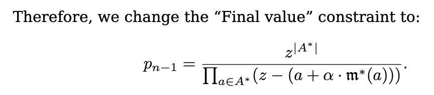
To do this, the first accesses are replaced with accesses to in . on the other hand uses acceses to the first parts of the memory and retrieves values from the public memory (e.g. ).
This means two things:
- the nominator of will contain in the first iterations (so ). Furthermore, these will not be cancelled by any values in the denominator (as is supposedly using actual accesses to the public memory)
- the denominator of will contain , and these values won’t be canceled by values in the nominator either
As such, the final value of the accumulator should look like this if the prover followed our directions:
which we can enforce (as the verifier) with a boundary constraint.
Section 9.8 of the Cairo paper writes exactly that:
CairoVM
Cairo compiles down to CairoVM and in the end produce a memory vector and execution trace table that is populated throughout the execution of the program.
More specifically, the fully assigned memory can be thought of as a vector that is divided into segments that have different functionalities (e.g. program instructions, execution, output). The execution trace is a table with 3 columns each representing a register value and rows that each represent the value of the registers over the execution of the program.
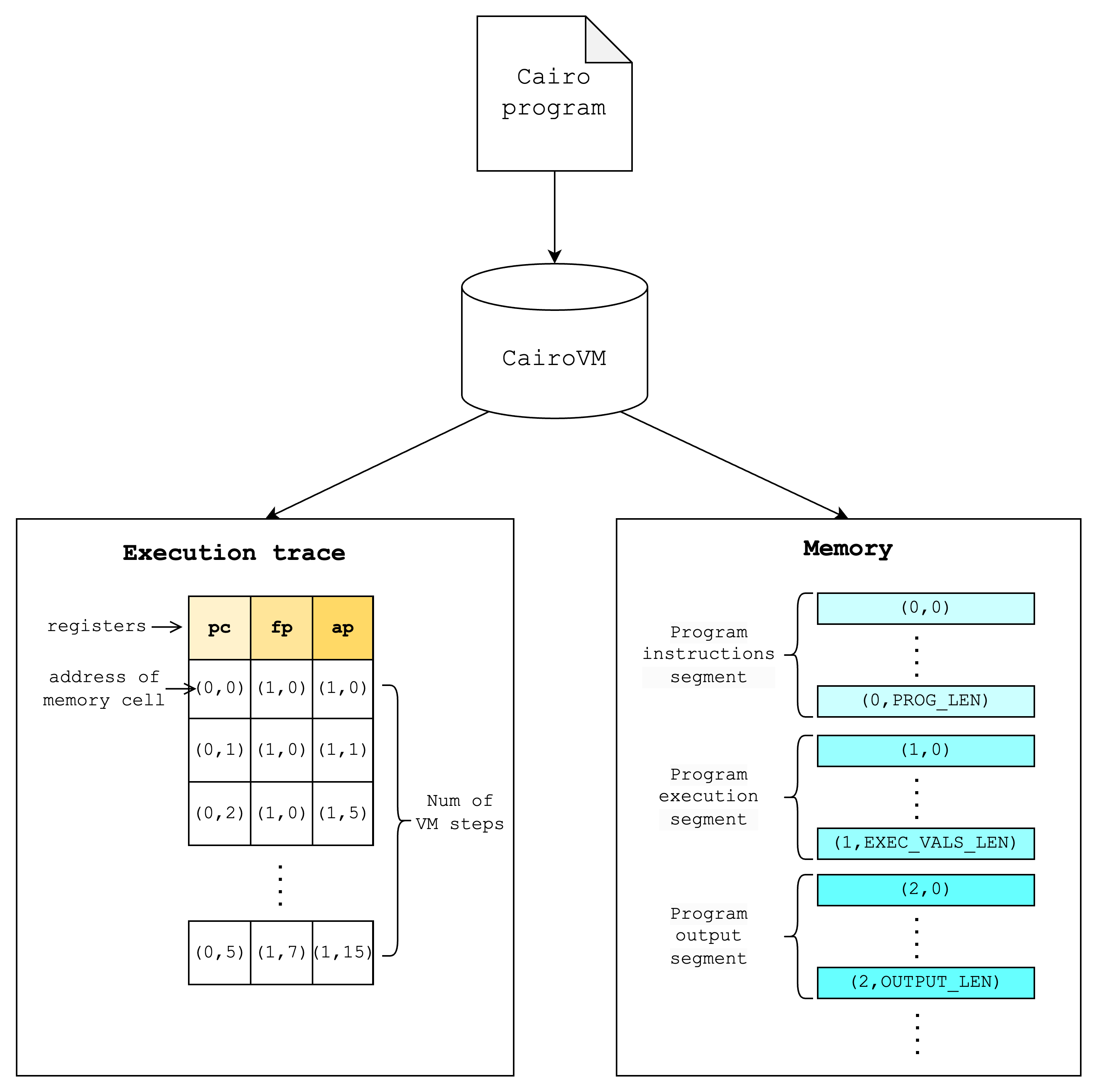
Note: the execution segment can be thought of as values that are written to the memory when running a program. Since the memory values can only be written once in CairoVM, Cairo programs keep track of the next available memory cell with a “allocation pointer” register (similar to a bump allocator in conventional terms).
Using these results of the CairoVM execution, the Stone prover can create a proof that proves the following (very roughly speaking):
- there exists a valid execution trace of n steps on the CairoVM
- which starts with a given set of initial register values
- which ends with a given set of final register values
- for some memory which satisfies certain constraints (e.g. read-only, continuous, consistent with the public memory portion)
Builtins
Builtins can be understood as memory-mapped peripherals, i.e. pre-allocated memory cells that can be used for certain commonly-used functions.
As of Cairo v0.13.1, these builtins are currently supported:
- Output
- Pedersen
- Range check (128 bits)
- Bitwise
- Elliptic curve operation
- Keccak
- Poseidon
- Range check (96 bits)
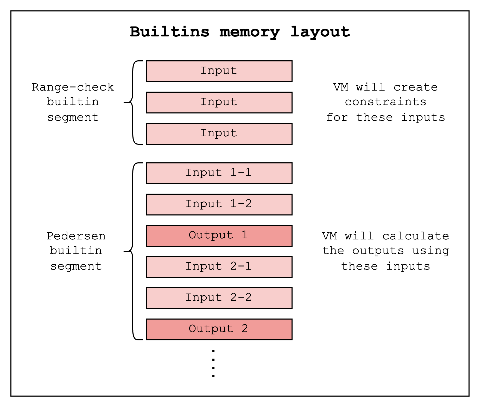
Each builtin is assigned a separate segment in the memory vector. The VM will write the builtin inputs to memory cells in the segment and retrieve the builtin outputs by reading memory cells from the segment.
For the range-check builtin, the CairoVM simply writes the value to be range checked into the next unused cell in the range-check segment. This segment guarantees that every memory cell in the range [X, Y).
For a Pedersen builtin, on the other hand, for each builtin use, you can input two values and read the next cell as output since the VM provides a guarantee that the next cell will contain the correct output (i.e. the Pedersen hash of the two input values).
In order to run a program that uses one of these builtins, we need to specify a specific layout to CairoVM that supports the builtins that the program uses. Below is a subset of layouts that are currently supported by the CairoVM. (Check this code for the updated, comprehensive list)
| small | recursive | dex | recursive_with_poseidon | starknet | starknet_with_keccak | |
|---|---|---|---|---|---|---|
| output | O | O | O | O | O | O |
| pedersen | O | O | O | O | O | O |
| range_check | O | O | O | O | O | O |
| bitwise | O | O | O | O | ||
| ecdsa | O | O | O | |||
| poseidon | O | O | O | |||
| ec_op | O | O | ||||
| keccak | O |
Hints
Hints are non-deterministic computation (i.e. code that is run outside of the VM to populate values that are validated inside the VM)
For example, when computing the square root of an integer in a prime field, directly computing this using constraints is expensive. So instead, we can use hint to calculate the square root and create a constraint inside the VM that checks that the power of the given square root is equal to the original value.
So given a computation , compute using a hint and create a constraint:
from the perspective of the VM is a wild guess, but the constraint makes sure that it’s valid.
In Cairo 0 language, you can run a hint by embedding a block of Python code. Below is an example of computing a square root of 25.
[ap] = 25, ap++;
%{
    import math
    memory[ap] = int(math.sqrt(memory[ap - 1]))
%}
[ap - 1] = [ap] * [ap], ap++;
When compiling this Cairo 0 program into CASM, the compiler stores this Python code as a string and specifies that this hint should be run before running the ensuing instruction. In this case, the hint should be run before the [ap - 1] = [ap] * [ap], ap++; instruction.
Bootloader
The primary purpose of the bootloader is to reduce the size of the public inputs, which includes the instructions of the program that is being proven. Since this can become a bottleneck once a program becomes big enough, the idea is to create a program of constant size that executes the big program and outputs only the hash of its instructions, which can be externally verified. Using the bootloader, we can also do the following: 1. sequentially run multiple programs, and 2. recursively verify bootloader proofs inside the bootloader.
Note: this doc is based on the Cairo v0.13.1 version of the bootloader
Please refer to the CairoVM doc for an overview of how CairoVM works.
How the “simple bootloader” works
Here is a pseudocode of how the simple bootloader works on a high level:
function run_simple_bootloader(tasks):
    load_bootloader_instructions()
    write_to_output(len(tasks))

    for task in tasks:
        load_task_instructions(task)
        hash = compute_task_instructions_hash(task)
        write_to_output(hash)

        builtin_pointers = get_required_builtin_allocators(task)
        task_outputs = run_task(task, builtin_pointers)
        write_to_output(task_outputs)

        for pointer in builtin_pointers:
            validate_allocator_advancement(pointer)

function validate_allocator_advancement(pointer):
    advancement = pointer.current_pointer - pointer.initial_pointer
    assert advancement >= 0 and advancement % pointer.cells_per_use == 0
Running the bootloader program (as running any Cairo program) will result in a memory vector and an execution trace. But since the bootloader program runs Cairo programs inside it, the generated memory and execution trace should include those of the Cairo programs as well. Below is an example of what the memory layout looks like after running the bootloader:
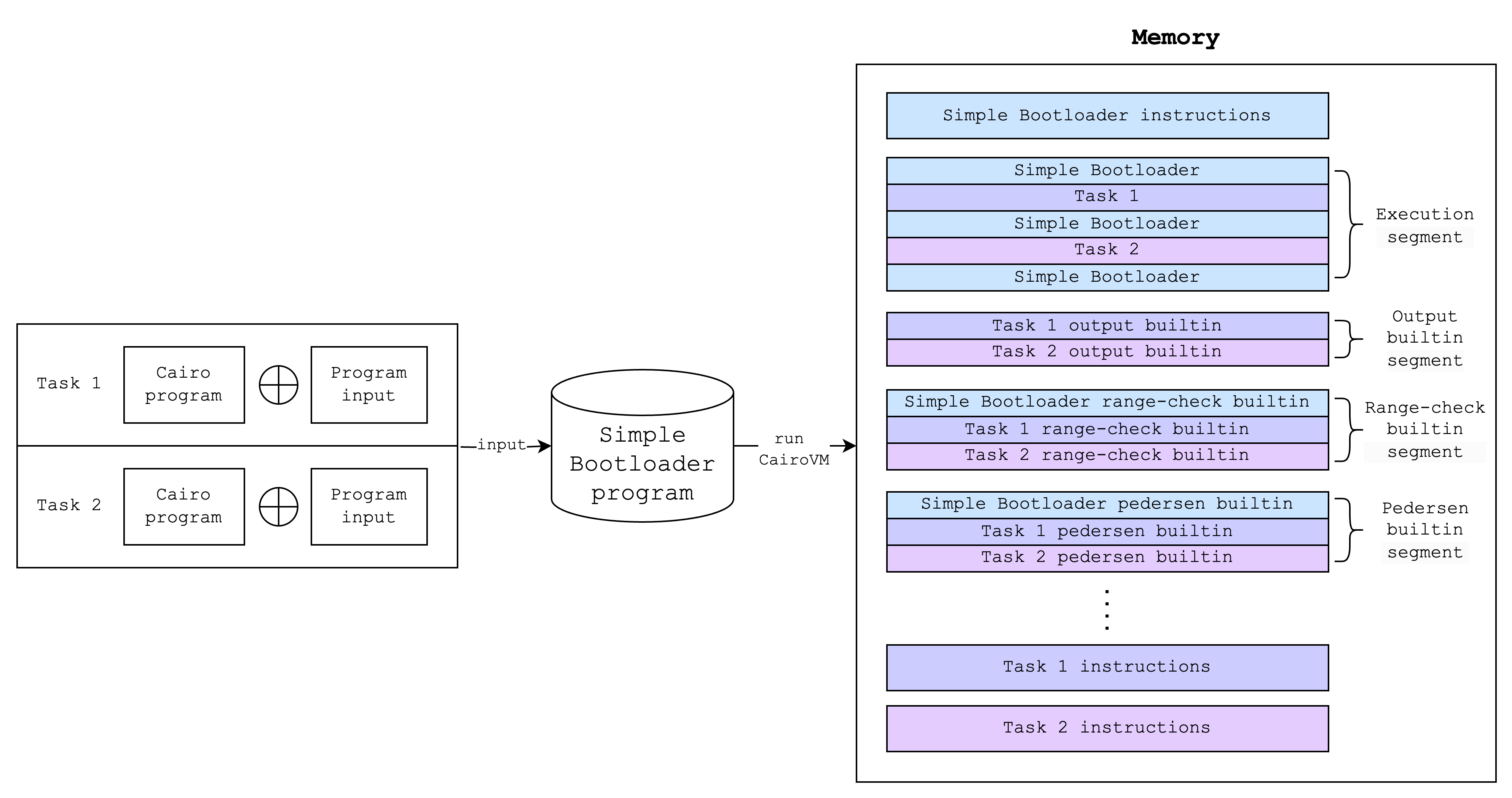
(Note: a task here refers to a single Cairo program and its inputs)
In other words, what the bootloader program does is it makes sure that the inner Cairo programs can write to various segments in the memory without any conflicts with each other or with the outer bootloader program. It also hashes the instructions of each inner Cairo program and writes the hashes to the output.
This is a “simple” use of the bootloader and we can use this functionality using the simple_bootloader.cairo file (link) in the Cairo repo. We will discuss an “advanced” use of the bootloader in the How the “advanced” bootloader works section.
Some more details on how the “simple” bootloader works
What builtins does the bootloader use?
-
output
- used to write the number of tasks and sequentially write the output related to each task
-
pedersen
- used to hash the task program bytecode
-
range checks
-
used to check that each task program used the builtins correctly.
-
Each builtin has a different amounts of memory cell usage
output=1, pedersen=3, range_check=1, ecdsa=2, bitwise=5, ec_op=7, keccak=16, poseidon=6, -
So for example, since the pedersen builtin requires 3 cells (2 for inputs, 1 for output), the bootloader checks that the difference between the pedersen builtin pointer before and after the task program run is positive (this is where the range check comes in) and that it is divisible by 3.
-
How are task program bytecode loaded into memory?
The bootloader creates a separate segment in the memory for storing each task program bytecode
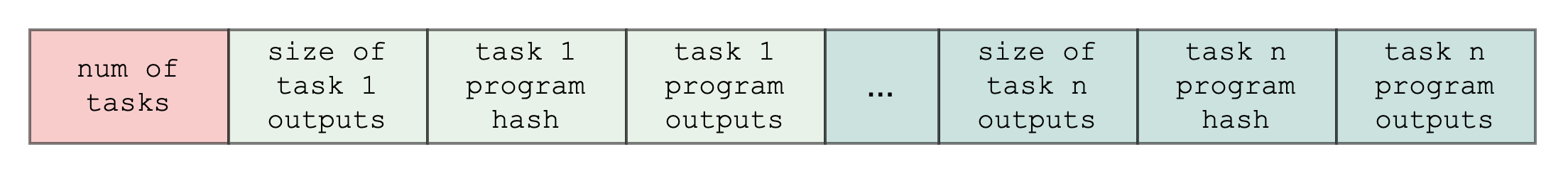
How are task outputs written to memory?
The bootloader writes the task outputs sequentially (i.e. in the order that the task programs are run) to the output builtin segment. Below is an example of what this looks like:
How do task programs use builtins other than the output builtin?
- assuming that the selected layout supports the builtins that the task program uses, the bootloader will pass the necessary builtin pointers to the task program’s main function, and the task program will use builtin cells as needed and return the pointers to the next unused builtin cells.
- at the end of the task program run, the bootloader will validate that the builtin pointers have been correctly advanced, as explained in the What builtins does the bootloader use? section.
How are task program hints handled?
- As mentioned in the A short primer on how the CairoVM works section, hints are specified to run before a certain bytecode is executed. In CairoVM, that refers the the “pc” value, or the program counter, and this value is normally a value in Segment 0. So a typical hint should run before, say when pc=(Segment 0, Index 15).
- However, task program bytecode are loaded into a separate segment (e.g. Segment 11), so the pc values for the hints of the task program need to updated accordingly.
How the “advanced” bootloader works
The “advanced” bootloader builds upon the “simple” bootloader by allowing as input not just Cairo programs but also a structured set of inputs that include both Cairo programs and simple bootloader proofs. In this section, we will go over how this works in multiple steps.
(The “advanced” bootloader refers to the bootloader.cairo file (link) in the Cairo repo.)
Step 1: A Cairo verifier program
First, we need to understand what a Cairo verifier program is.
A Cairo verifier is a Cairo program that verifies a Cairo proof, and in this case, it will only verify a proof generated using the “simple” bootloader. Below is an example of what running a Cairo verifier program looks like.
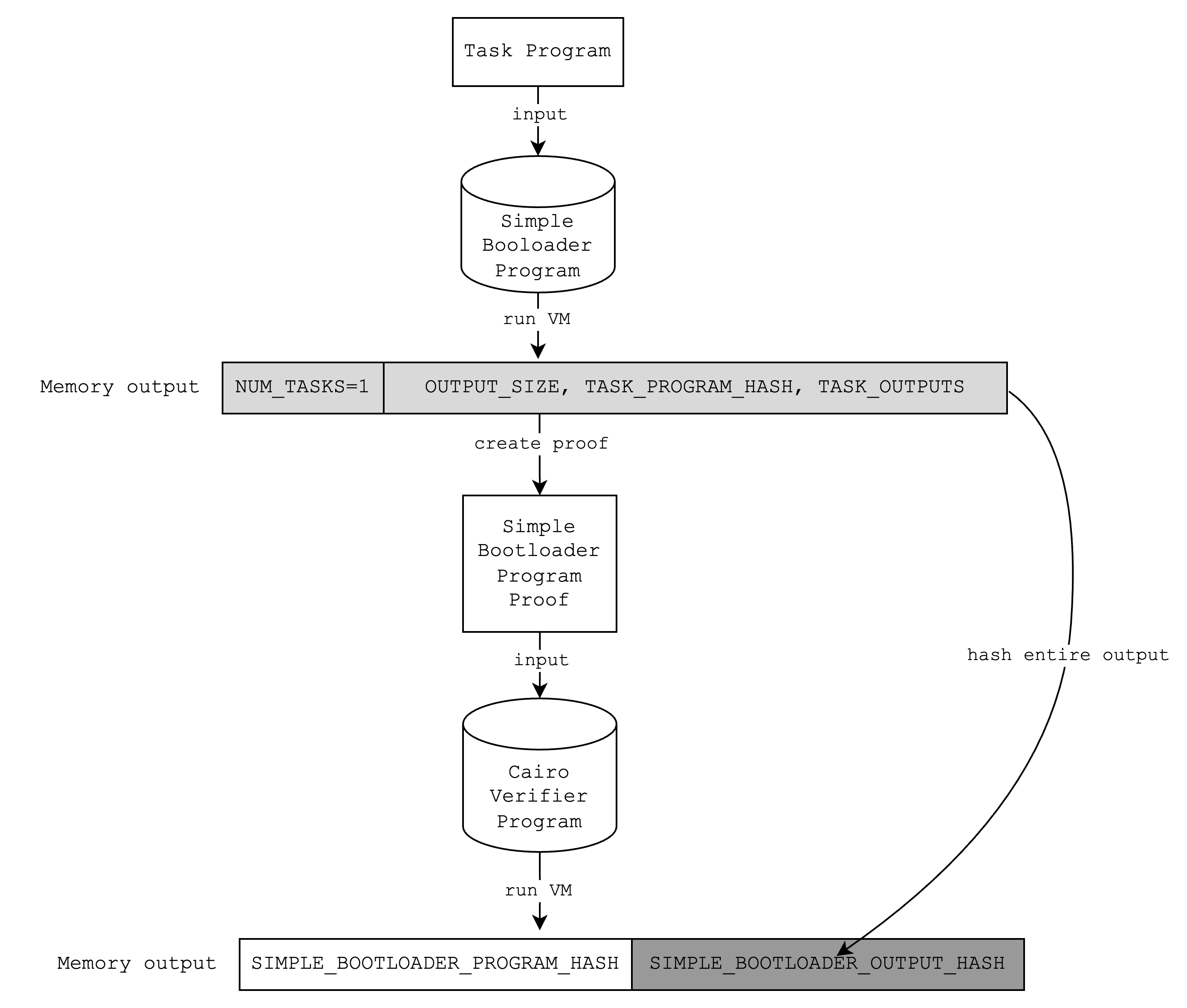
Note that when the Cairo verifier verifies the simple bootloader proof, it includes in the output the hash of the simple bootloader program and the hash of the outputs of the simple bootloader. This means that it is possible to commit to the output of the simple bootloader using the Cairo verifier and open it later.
Step 2: Iteratively creating proofs
Looking closely at diagram above, you can see that we can tweak it a little bit to create a perfect loop. Since the simple bootloader can run any arbitrary program and the Cairo verifier requires a proof of the simple bootloader, we can do something like the following:
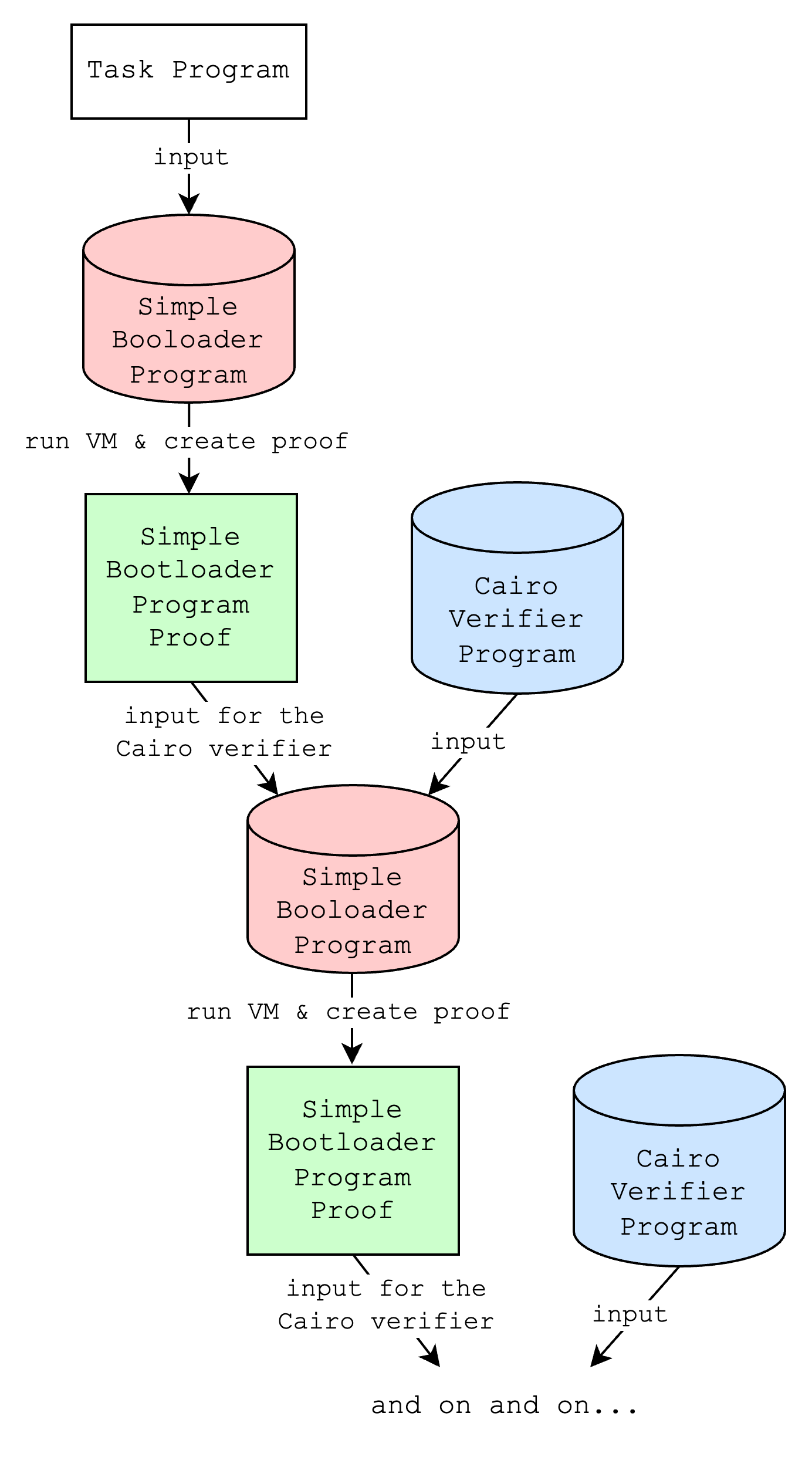
Of course, there is no point in just repeating this loop, but if we tweak this just a little bit again, we can do something more interesting: creating a proof that both verifies an existing proof and proves a new program. We’ll call this “iteratively creating proofs”, which is the core of what the “advanced” bootloader does.
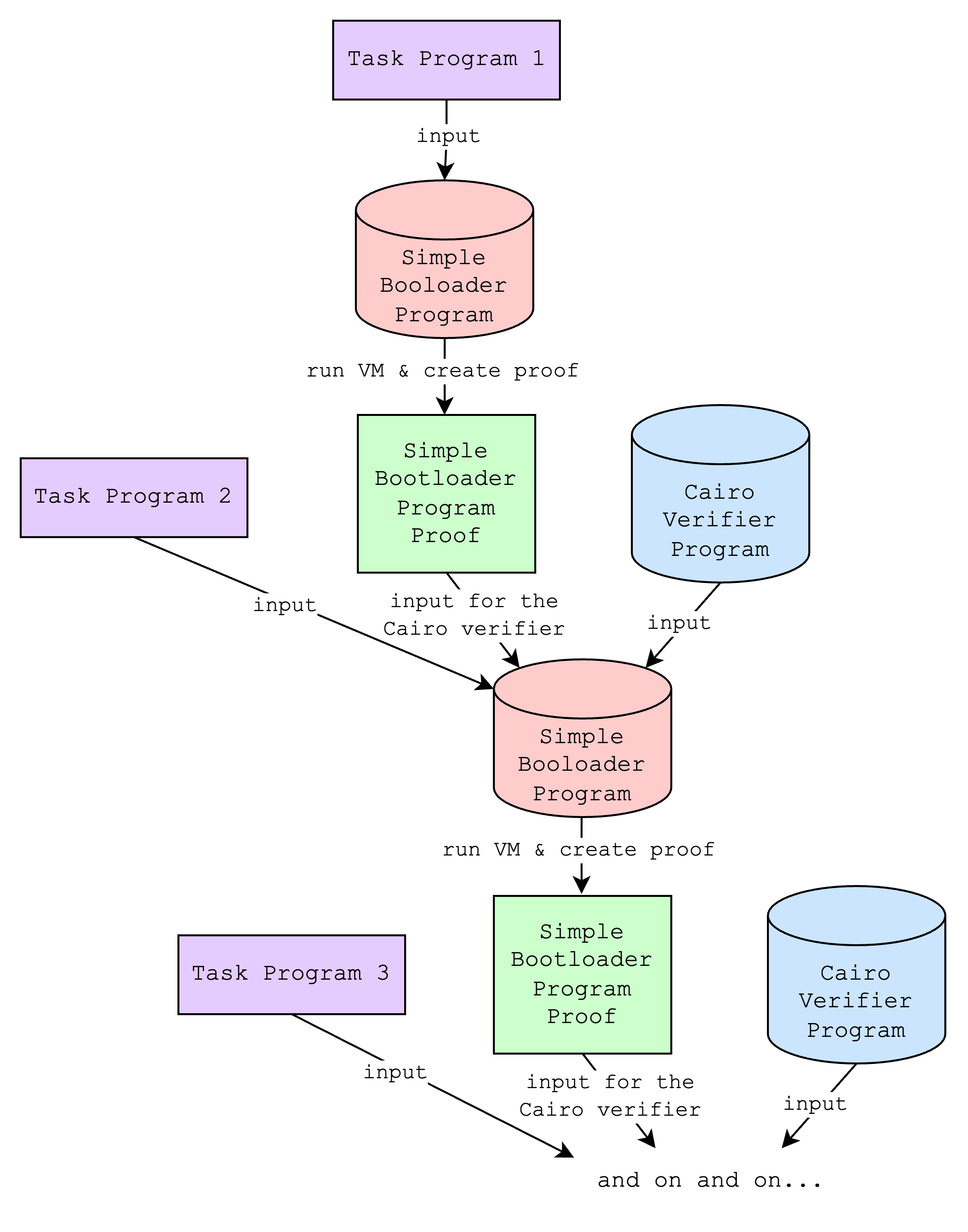
This might still not seem too useful, but it unlocks a new use case for users who want to create proofs of programs as they come, not just when they have a fixed set. For example, L2 nodes that need to create a single proof of programs that are transmitted over a 15-minute period do not need to wait for the whole 15 minutes and create a proof at the last minute, which would take a long time if the number of programs to be proven are large. Instead, they can create a proof after the first 1 minute, and for the next 14 times every minute they can create a new proof that recursively proves the previous proof and proves the new programs.
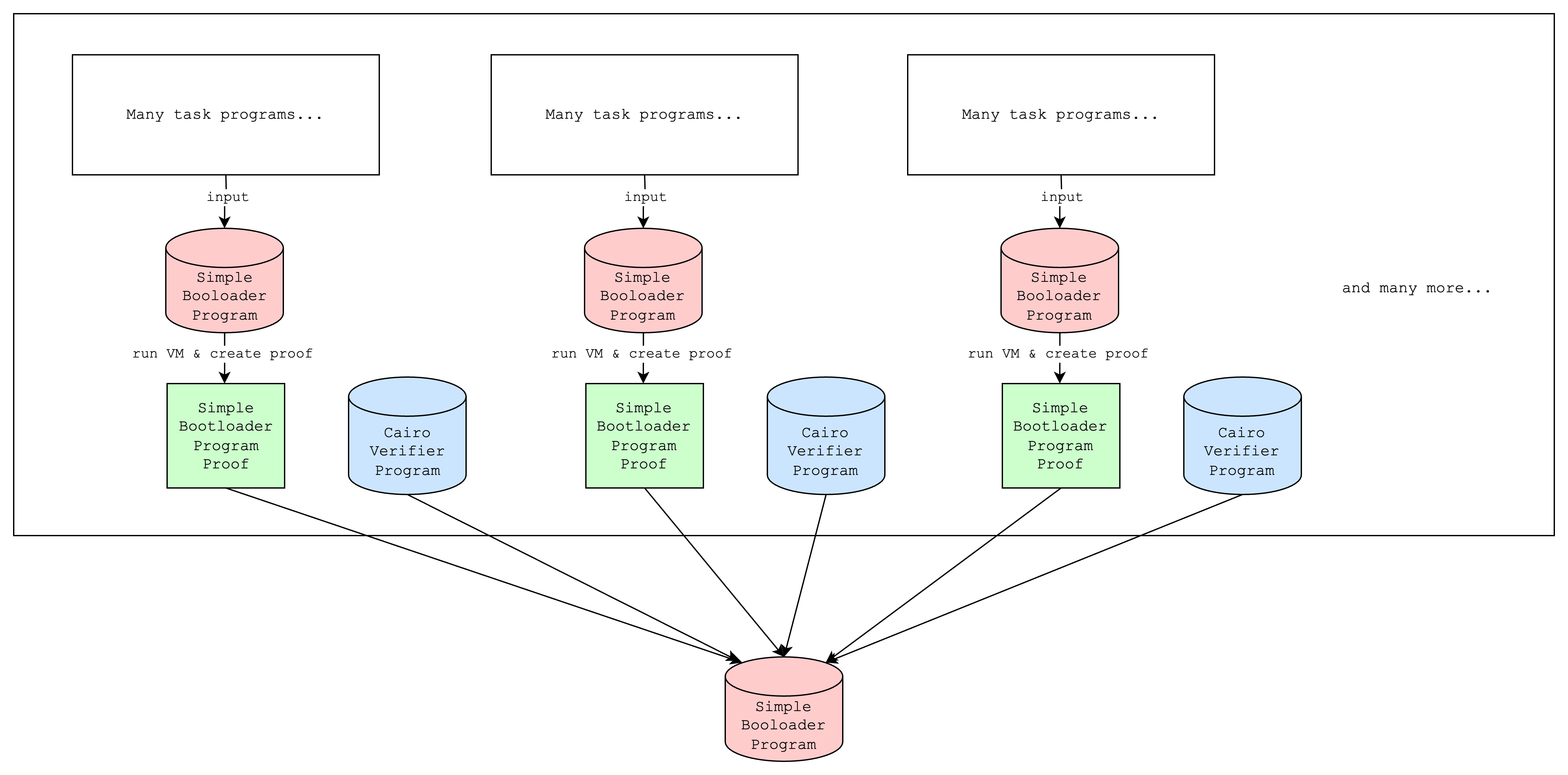
We can also simply run multiple simple bootloaders on separate programs and aggregate the proofs with a single additional simple bootloader execution. This can have the following benefits:
- improve proving time if multiple simple bootloaders are run in parallel
- avoid memory limits from proving too many programs at once
Step 3: Verifying iteratively created proofs
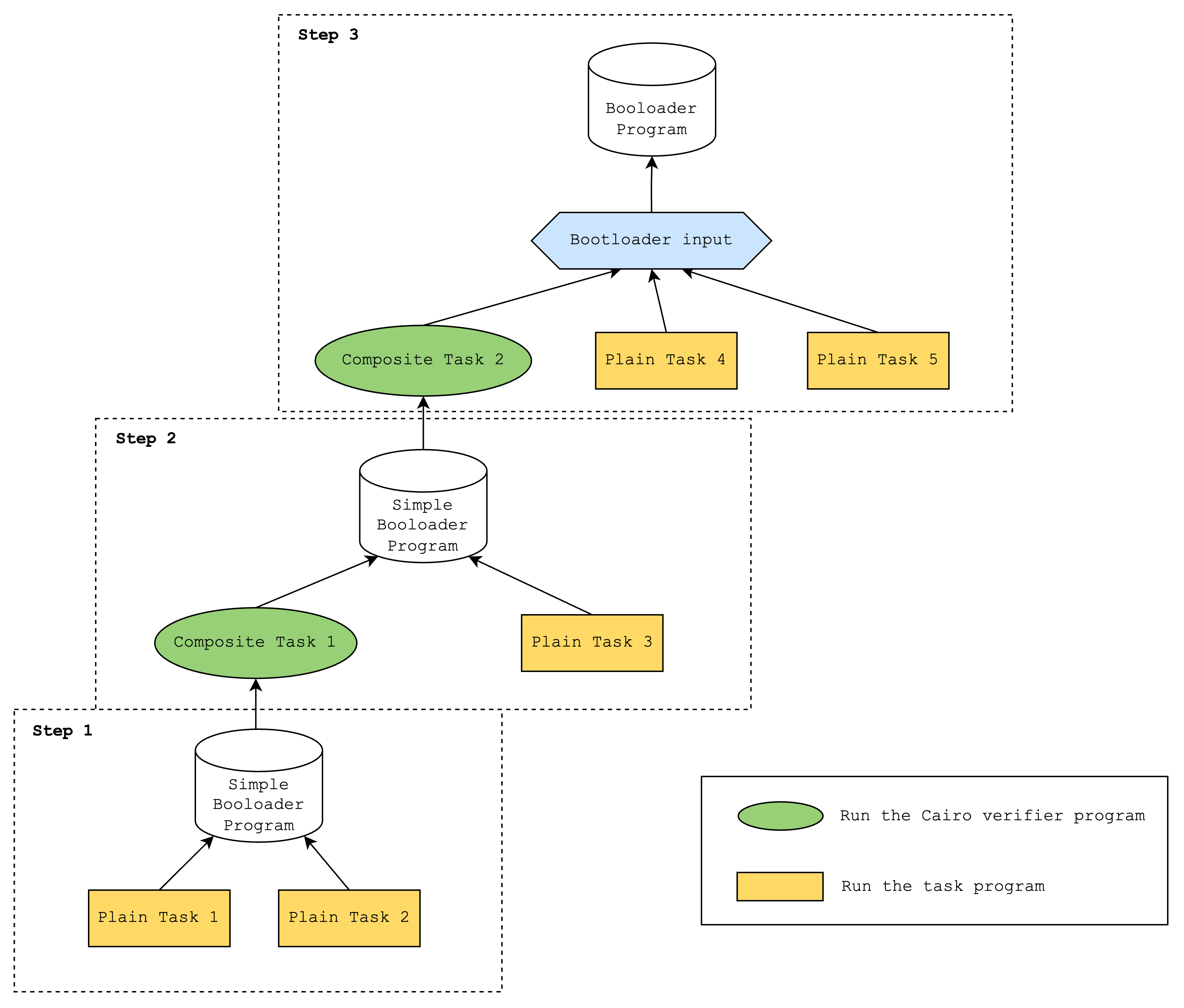
At the end of the iterations, we will have a simple bootloader program proof but its output will be a hash of the outputs of the previous iteration (as mentioned in Step 1). We can view this as a tree where the output of the final iteration is the root.
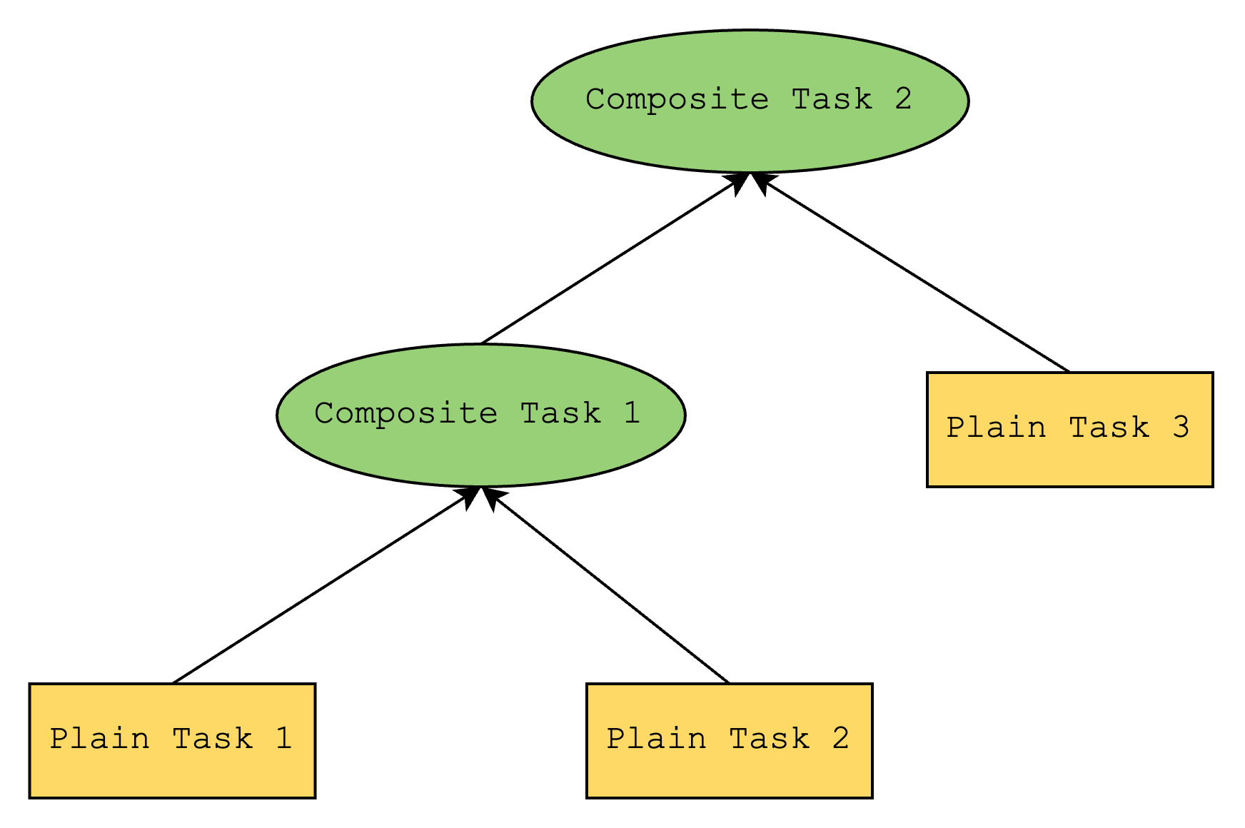
So the tree will look something like the above, where a plain task represents a Cairo program and a composite task represents a Cairo verifier program. Here, Composite Task 2 represents the root of the tree, and it contains the hash of the outputs of Composite Task 1 and Plain Task 3.
Unfortunately, the simple bootloader does not have a way to verify that this root is correct, and this is where the “advanced” bootloader steps in. The “advanced” bootloader verifies the root by doing a depth-first search and verifying that all internal nodes (i.e. composite tasks) correctly hash the outputs of its children.
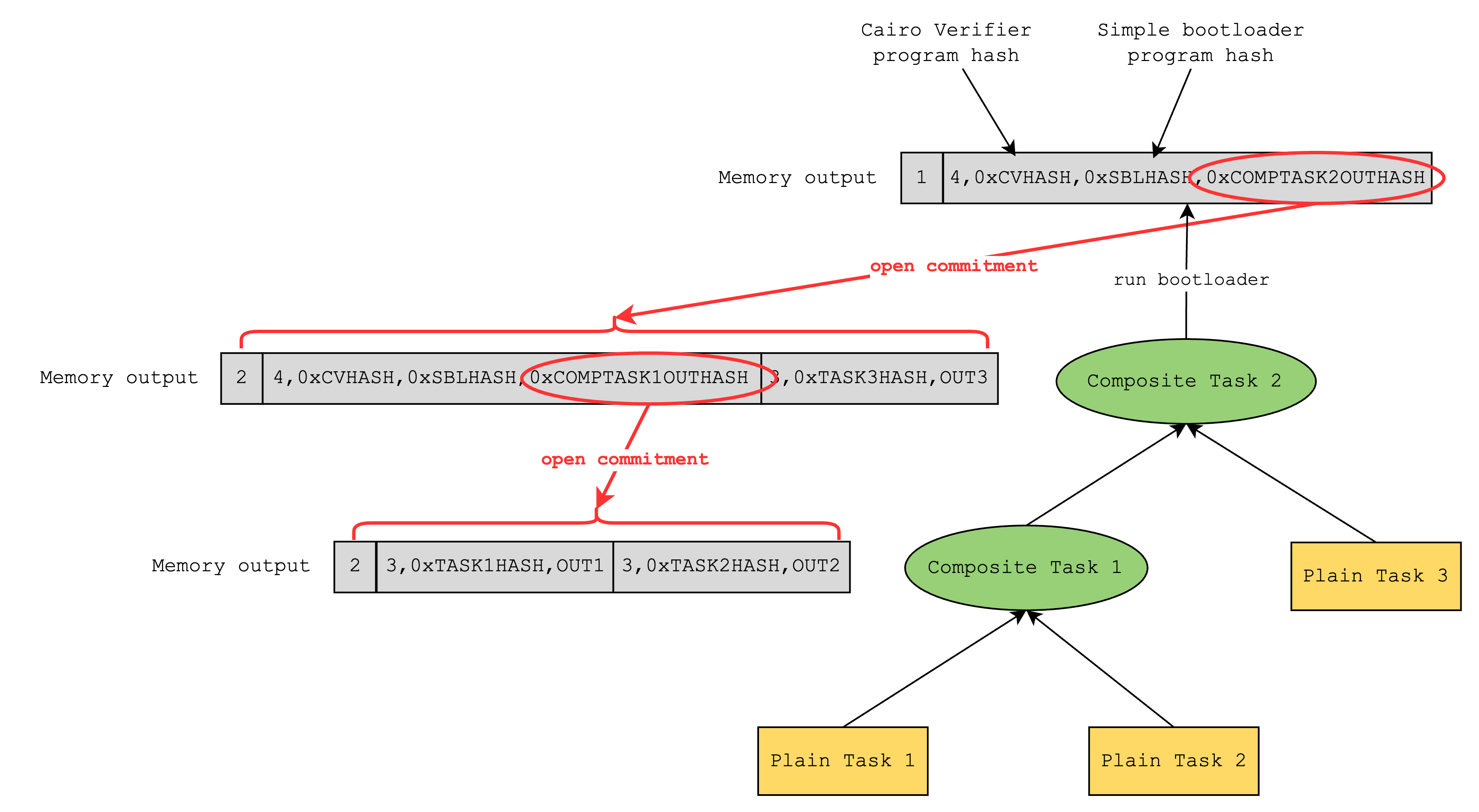
After verification, the advanced bootloader now knows all the leaf data of the tree, so it can write to the output the entire set of task program outputs that have been proven throughout the iterations. This way, anyone looking at the bootloader output can check that a certain Cairo program has a certain output.

Bringing it all together, this is what a sample bootloader run looks like:
- Run simple bootloader that runs Plain Task 1 and Plain Task 2
- Run simple bootloader that runs Composite Task 1 and Plain Task 3
- Run advanced bootloader that runs Composite Task 2 and Plain Task 4 and Plain Task 5
In step 3, the outputs of Plain Tasks 1, 2, and 3 will need to be provided as hints to the advanced bootloader.
Builtins and Layouts
Builtins
Layouts
Different layouts are deployed on SHARP:
https://github.com/starkware-libs/starkex-contracts/tree/aecf37f2278b2df233edd13b686d0aa9462ada02/evm-verifier/solidity/contracts/cpu
Starkex
The starkex contracts are:
- deployed at 0x6cB3EE90C50a38A0e4662bB7e7E6e40B91361BF6
- and sit behind the upgradable smart contract at 0x47312450b3ac8b5b8e247a6bb6d523e7605bdb60.
By looking at the Constructor Arguments section of the implementation contract (which might be outdated at the moment of this writing, as the implementation contract is upgradable) one can see where the subcontracts are deployed:
bootloaderProgramContract: 0x5d07afFAfc8721Ef3dEe4D11A2D1484CBf6A9dDfmemoryPageFactRegistry_: 0xFD14567eaf9ba941cB8c8a94eEC14831ca7fD1b4cairoVerifierContracts]: 0x217750c27bE9147f9e358D9FF26a8224F8aCC214,0x630A97901Ac29590DF83f4A64B8D490D54caf239,0x8488e8f4e26eBa40faE229AB653d98E341cbE57B,0x9E614a417f8309575fC11b175A51599661f2Bd21,0xC879aF7D5eD80e4676C203FD300E640C297F31e3,0x78Af2BFB12Db15d35f7dE8DD77f29C299C78c590,0xe9664D230490d5A515ef7Ef30033d8075a8D0E24,0x03Fa911dfCa026D9C8Edb508851b390accF912e8hashedSupportedCairoVerifiers:3178097804922730583543126053422762895998573737925004508949311089390705597156simpleBootloaderProgramHash:2962621603719000361370283216422448934312521782617806945663080079725495842070
Note: The different verifier contracts correspond to the different layouts that are supported for Cairo (see the Builtins and Layouts of Cairo section of the book).
Somewhat outdated implementations live on Github at starkware-libs/starkex-contracts.
They implement the SHARP (SHARed Prover) verifier, which allows us to verify SHARP proofs on Ethereum.
Note: A number of contracts refer to “GPS” which is the old name for SHARP (general-proving service).
Any application on Ethereum that wants to use Cairo can make use of this service to verify proofs. The flow is split in two parts:
- The proof is sent to the SHARP service, which verifies it and returns a fact.
- The application can check that the fact has been verified.
We explain what “facts” are in facts section.
Fact Registry
The Starkex contracts implement the verifier side of the SHARP service. In other words, when people create proofs using the SHARP service, they can get them verified on Ethereum using the Starkex contracts.
First, let’s introduce what a fact is: a fact can be any computation that was computed by some logic in the smart contract. For example, a fact can be: “we successfully verified a proof for this Cairo program and these public inputs”. This example is actually the main fact that Starkex will register for the different applications making use of it. But internally, other facts are used whenever a computation (like verifying a proof) is split in different transactions that need to produce a snapshot of what has been done so far and resume from other snapshots. This is explained in more details in the Verifying Cairo proofs section.
A fact is represented (or authenticated) by a hash of its variables. As such, it is important that different applications or different contexts use “different” hash functions not to have collisions. This can be done by adding some domain separation string to the hash function, or as it is done by starkex by using different fact registries for different usecases.
The Fact Registry
Let’s introduce the smart contract in charge of these facts, FactRegistry.sol:
contract FactRegistry is IQueryableFactRegistry {
    // Mapping: fact hash -> true.
    mapping(bytes32 => bool) private verifiedFact
As you can see, facts are just tracked via a hashmap. Registering a fact is such straightfoward:
    function registerFact(bytes32 factHash) internal {
        // This function stores the fact hash in the mapping.
        verifiedFact[factHash] = true;
As well as checking if a fact has been registered:
    function isValid(bytes32 fact) external view override returns (bool) {
        return _factCheck(fact);
    }
Example of facts from external applications
An example of registering a fact can be seen, for example at the end of a proof verification. In GpsStatementVerifier.sol:verifyProofAndRegister():
    function verifyProofAndRegister(
        uint256[] calldata proofParams,
        uint256[] calldata proof,
        uint256[] calldata taskMetadata,
        uint256[] calldata cairoAuxInput,
        uint256 cairoVerifierId
    ) external {
        // TRUNCATED...

        registerGpsFacts(taskMetadata, publicMemoryPages, cairoAuxInput[OFFSET_OUTPUT_BEGIN_ADDR]);
    }
where registerGpsFacts is defined as:
    function registerGpsFacts(
        uint256[] calldata taskMetadata,
        uint256[] memory publicMemoryPages,
        uint256 outputStartAddress
    ) internal {
        // TRUNCATED...

        // Register the fact for each task.
        for (task = 0; task < nTasks; task++) {
            // TRUNCATED...

            bytes32 fact = keccak256(abi.encode(programHash, programOutputFact));

            // TRUNCATED...
            registerFact(fact);

            // TRUNCATED...
        }

        // TRUNCATED...
    }
Starknet is the main application making use of SHARP, and as such their smart contract uses the fact registry directly.
The main function of Starknet is updateState(), which updates the state based on proofs that have been verified:
    function updateState(
        int256 sequenceNumber,
        uint256[] calldata programOutput,
        uint256 onchainDataHash,
        uint256 onchainDataSize
    ) external onlyOperator {
        // TRUNCATED...

        bytes32 sharpFact = keccak256(
            abi.encode(programHash(), stateTransitionFact)
        );
        require(
            IFactRegistry(verifier()).isValid(sharpFact),
            "NO_STATE_TRANSITION_PROOF"
        );

        // TRUNCATED...
Example of checking if a fact internally
Another example we can look at is within a proof verification. As explained in Verifying a Cairo proof, a proof verification is split in multiple transactions.
For example, Merkle membership proofs are verified in segregated transactions, and then the fact that they were verified is used within another execution. The fact is first verified and then registered in MerkleStatementContract:verifyMerkle():
    function verifyMerkle(
        uint256[] memory merkleView,
        uint256[] memory initialMerkleQueue,
        uint256 height,
        uint256 expectedRoot
    ) public {
        // TRUNCATED...

        bytes32 resRoot = verifyMerkle(channelPtr, merkleQueuePtr, bytes32(expectedRoot), nQueries);
        bytes32 factHash;
        assembly {
            // Append the resulted root (should be the return value of verify) to dataToHashPtr.
            mstore(dataToHashPtr, resRoot)
            // Reset dataToHashPtr.
            dataToHashPtr := add(channelPtr, 0x20)
            factHash := keccak256(dataToHashPtr, add(mul(nQueries, 0x40), 0x20))
        }

        registerFact(factHash);
    }
and in MerkleStatementVerifier:verifyMerkle():
    function verifyMerkle(
        uint256, /*channelPtr*/
        uint256 queuePtr,
        bytes32 root,
        uint256 n
    ) internal view virtual override returns (bytes32) {
        // TRUNCATED...

        require(merkleStatementContract.isValid(statement), "INVALIDATED_MERKLE_STATEMENT");
        return root;
    }
where both use their own fact registry not to collide with other usecase (as pointed out at the beginning of this section).
Verifying Cairo proofs
Verifying a SHARP Cairo proof on the Starkex contracts is done in a number of transactions:
- 3 Verify Merkle transactions to verify Merkle paths (example)
- 8 Verify FRI transactions to verify the FRI proofs (example)
- A bunch of Register Continuous Memory Page transactions (example)
- A single Verify Proof and Register (example)
The reason the verification of a proof is split in multiple transactions is because proofs are too large, and the verification cost too much gas, to fit in a single transaction.
Note: Proofs can be split using stark-evm-adapter
Layouts
Different layouts are deployed on SHARP:
https://github.com/starkware-libs/starkex-contracts/tree/aecf37f2278b2df233edd13b686d0aa9462ada02/evm-verifier/solidity/contracts/cpu
Proof Splitter
Due to the gas limitations when verifying an original STARK proof, the proof generated by the Stone Prover should be split into three types: the main proof, Trace Merkle proof, and FRI proof. Typically, this includes one Main Proof accompanied by several Trace Merkle Proofs and FRI Proofs.
This process relies on the fact registry, which functions as verification snapshots. These snapshots can be viewed as pre-verified subproofs. This allows the Main Proof to be verified based on earlier snapshots obtained from the Merkle Proofs and FRI Proofs, thereby circumventing the bottleneck caused by gas limitations in a single EVM transaction.
This section aims to clarify the roles of the various proof types, showing how the split proof works with references to the source code in Cairo verifier contracts, Stone Prover and Stark EVM Adapter.
Main proof
The Main proof is the primary proof that corresponds to the original proof generated by the Stone Prover. It encompasses essential proof data, including commitments for traces and FRI layers, along with trace values necessary for deriving the deep composition polynomial , among other elements.
At a high level, it performs the following two key functions:
- Deriving a deep composition polynomial
- Checking FRI layers for
This explanation reuses the notations from the ethSTARK paper.
The Main Proof contains the commitments for the traces and FRI, as well as the trace values for deriving the polynomial .
These trace values, also referred to as mask values, can be categorized into two types:
- Trace values involved in expressing in the following composition polynomial:
- Evaluations of the polynomials decomposed from the :
By invoking the CpuConstraintPoly contract to evaluate the with the trace mask values, it checks the out-of-domain-sampling (oods) consistency among these provided trace values and the evaluations of decomposed composition polynomial.
In other word, to do the check at a random point , they check:
After passed the OODS consistency check, it proceeds to prepare and verifie the FRI layers for .
By aggregating the trace values and evaluations obtained from the OODS, it derives the deep composition polynomial (or quotient polynomial) through the CpuOods contract.
FRI plays the role as a PCS. Doing this means that the prover has to prove that quotient polynomial exists for OODS evaluations and is of degree . During FRI the verifier will obtain different evaluations of . For example if they want an evaluation of the prover would have to produce merkle proofs for for all and for all .
In the first FRI layer computation stage, the contract reads these induced values based on FRI queries and decommits them from the main proof. Three traces are required for the Cairo verifier: execution trace, interaction trace and composition trace. Each decommitment checks against a trace commitment, which should have been verified and registered as a fact in the Merkle fact registry.
These facts serve as verification snapshots, which are crucial when it is needed to split a verification into multiple stages. This approach is necessary due to various reasons, such as circumventing gas cost limitations or conserving gas costs for transaction retries based on a verified snapshot.
Similarly, the process of checking the FRI layers depends on the FRI Merkle verification snapshots obtained earlier. It involves verifying whether the fact is registered with the FRI layer’s commitment.
Other split proofs
In order to provide the verfication snapshots for the Main Proof, it is essential to first complete both the Trace Merkle Proofs and the FRI Merkle Proofs. These preliminary steps are necessary to generate the verification snapshots required for the Main Proof.
The MerkleStatementContract and FriStatementContract are specifically designed for verifying the Trace Merkle Proofs and FRI Merkle Proofs, respectively. Upon successful verification, these facts will be registered as verification snapshots.
Proof annotations
With the original proof file obtained from the Stone Prover, it is necessary to run its CPU verifier to generate the annotations. This process is akin to operating an offline simulator, which verifies the proof and simulates the required proof data as annotations. These annotations are then utilized by verifiers in other locations, such as the EVM Cairo verifier.
The primary reason for generating these annotations, rather than extracting directly from the original proof, would be to facilitate the restructuring of the data in the original proof into a clearer format. This restructuring is particularly beneficial for other verification procedures, such as those employed by EVM Cairo verifiers.
Here is an example of an annotated proof. This example showcases how annotations are combined with the original proof into a single JSON file for further processing. The annotations themselves represent various data points, here are some of the examples:
// execution trace commitment
"P->V[0:32]: /cpu air/STARK/Original/Commit on Trace: Commitment: Hash(0x3c8537043a0e5298ac50fd0c85a697b4f64ad84d000000000000000000000000)"
// interaction trace commitment
"P->V[32:64]: /cpu air/STARK/Interaction/Commit on Trace: Commitment: Hash(0xf5a5807d04f92b370a2ca27ccafaf40f196a27ab000000000000000000000000)"
// composition trace commitment
"P->V[64:96]: /cpu air/STARK/Out Of Domain Sampling/Commit on Trace: Commitment: Hash(0x2a0d752d3cf399e94ebc1cc8a425ce89d848b7d7000000000000000000000000)"
// verifier challenges for interaction trace
"V->P: /cpu air/STARK/Interaction: Interaction element #0: Field Element(0x29767aebd00e6750d36470c07b003624f52e08794f24c23c17fdbcf66e1593f)",
"V->P: /cpu air/STARK/Interaction: Interaction element #1: Field Element(0x5e8b64f90ebe7e15559196630cd2bb6bb95b0d9121ff82adf708a2e6637b142)..."
// oods evaluation point
"V->P: /cpu air/STARK/Out Of Domain Sampling/OODS values: Evaluation point: Field Element(0x4f03c43ef1a1476cea9b31c4880f1808ed0dada6e2d650af829115186740856)"
// commitments for FRI layers
"P->V[8768:8800]: /cpu air/STARK/FRI/Commitment/Layer 1: Commitment: Hash(0x994586a93d3f0397b588be7eb5ea55ecaec10145000000000000000000000000)",
"V->P: /cpu air/STARK/FRI/Commitment/Layer 2: Evaluation point: Field Element(0x69d6218dda1b690e11974c0d7bce4b5fb6584f5b188d2d8988436c9d7423fac)",
"P->V[8800:8832]: /cpu air/STARK/FRI/Commitment/Layer 2: Commitment: Hash(0x533a5b9d2896a3a50338eba17f3c660f6fc89995000000000000000000000000..."
Open source library
The Stark EVM Adapter provides an API to facilitate the splitting of original proofs from the Stone Prover into these segmented proofs. This library is particularly useful for developers working with STARK proofs in EVM environments. Included in the repository is a demo script that illustrates the complete process of splitting a Stone proof. This script demonstrates not only how to split the proof but also how to submit the resultant proofs to the Cairo verifier contracts.
Bootloader
Starknet
See more: https://book.starknet.io/