Evaluating Constraints Over Trace Polynomials

Proving Spreadsheet Functions

When we want to perform computations over the cells in a spreadsheet, we don't want to manually fill in the computed values. Instead, we leverage spreadsheet functions to autofill cells based on a given computation.

We can do the same thing with our table, except in addition to autofilling cells, we can also create a constraint that the result was computed correctly. Remember that the purpose of using a proof system is that the verifier can verify a computation was executed correctly without having to execute it themselves? Well, that's exactly why we need to create a constraint.

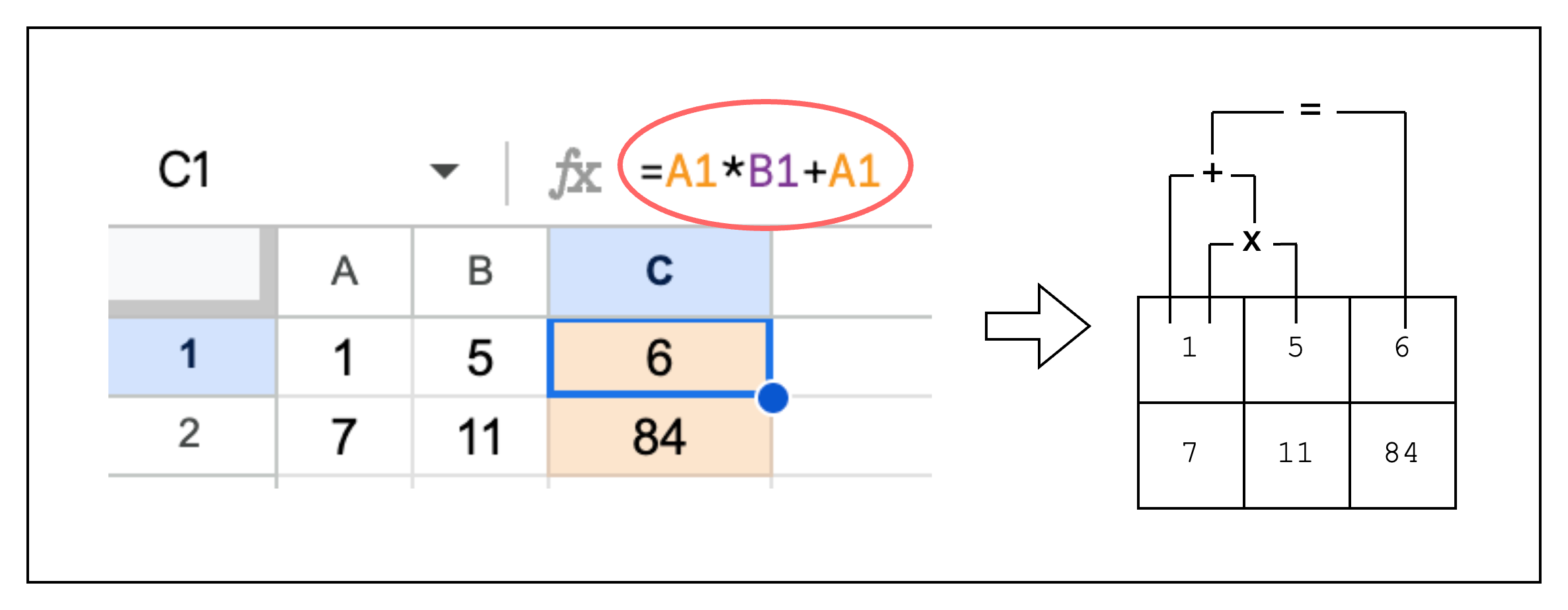
Now let's say we want to add a new column C to our spreadsheet that computes the product of the previous columns plus the first column. We can set C1 as A1 * B1 + A1 as in Figure 2.

In the same vein, we can create a new column in our table that computes the sum of the two previous columns. And we can constrain the value of the third column by creating an equation that must equal 0: col1_row1 * col2_row1 + col1_row1 - col3_row1 = 0.

Identical Constraints Every Row

Obviously, as can be seen in Figure 2, our new constraint is satisfied for every row in the table. This means that we can substitute creating a constraint for each row with a single constraint over the columns, i.e. the trace polynomials.

Thus, col1_row1 * col2_row1 + col1_row1 - col3_row1 = 0 becomes \(f_1(x) \cdot f_2(x) + f_1(x) - f_3(x) = 0\).

Composition Polynomial

We will now give a name to the polynomial that expresses the constraint: a composition polynomial.

\(C(x) = f_1(x) \cdot f_2(x) + f_1(x) - f_3(x)\)

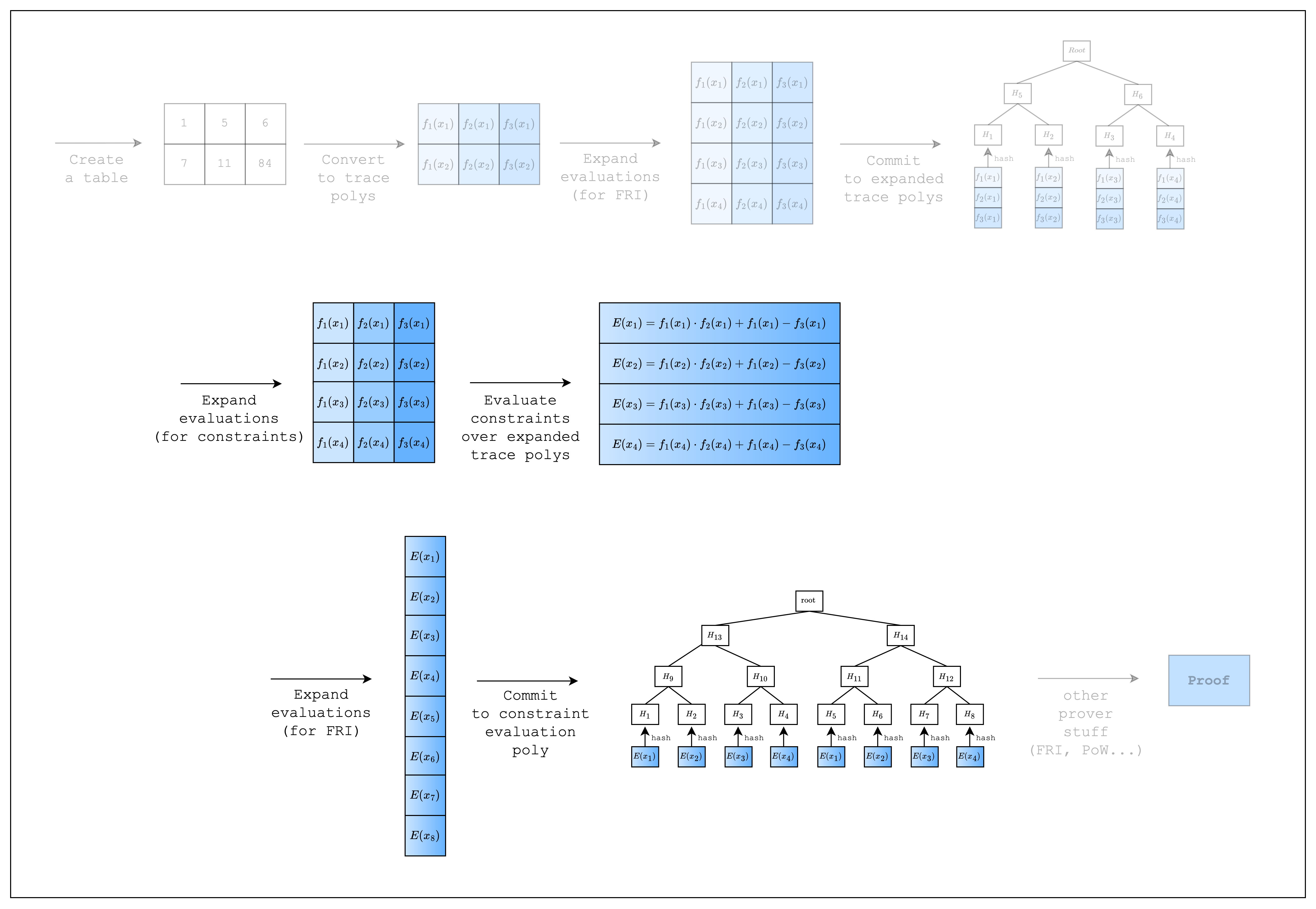
Basically, in order to prove that the constraints are satisfied, we need to show that the composition polynomial evaluates to 0 over the original domain (i.e. the domain of size the number of rows in the table).

But first, as can be seen in Figure 1, we need to expand the evaluations of the trace polynomials by a factor of 2. This is because the composition polynomial has degree 2, while the trace polynomials have degree 1, and thus we need more evaluations to uniquely determine the Lagrange polynomial.

Once we have the expanded evaluations, we can evaluate the composition polynomial. Checking that the composition polynomial evaluates to 0 over the original domain is done in FRI, so once again we need to expand the composition polynomial evaluations by a factor of 2 and commit to them.

We'll see in the code below how this is implemented.

Code

struct TestEval {
    log_size: u32,
}

impl FrameworkEval for TestEval {
    fn log_size(&self) -> u32 {
        self.log_size
    }

    fn max_constraint_log_degree_bound(&self) -> u32 {
        self.log_size + CONSTRAINT_EVAL_BLOWUP_FACTOR
    }

    fn evaluate<E: EvalAtRow>(&self, mut eval: E) -> E {
        let col_1 = eval.next_trace_mask();
        let col_2 = eval.next_trace_mask();
        let col_3 = eval.next_trace_mask();
        eval.add_constraint(col_1.clone() * col_2.clone() + col_1.clone() - col_3.clone());
        eval
    }
}

fn main() {
    // --snip--

    let mut col_3 = BaseColumn::zeros(num_rows);
    col_3.set(0, col_1.at(0) * col_2.at(0) + col_1.at(0));
    col_3.set(1, col_1.at(1) * col_2.at(1) + col_1.at(1));

    // Convert table to trace polynomials
    let domain = CanonicCoset::new(log_num_rows).circle_domain();
    let trace: ColumnVec<CircleEvaluation<SimdBackend, M31, BitReversedOrder>> =
        vec![col_1, col_2, col_3]
            .into_iter()
            .map(|col| CircleEvaluation::new(domain, col))
            .collect();

    // --snip--

    // Create a component
    let _component = FrameworkComponent::<TestEval>::new(
        &mut TraceLocationAllocator::default(),
        TestEval {
            log_size: log_num_rows,
        },
        QM31::zero(),
    );
}

First, we add a new column col_3 that contains the result of the computation: col_1 * col_2 + col_1.

Then, to create a constraint over the trace polynomials, we first create a TestEval struct that implements the FrameworkEval trait. Then, we add our constraint logic in the FrameworkEval::evaluate function. Note that this function is called for every row in the table, so we only need to define the constraint once.

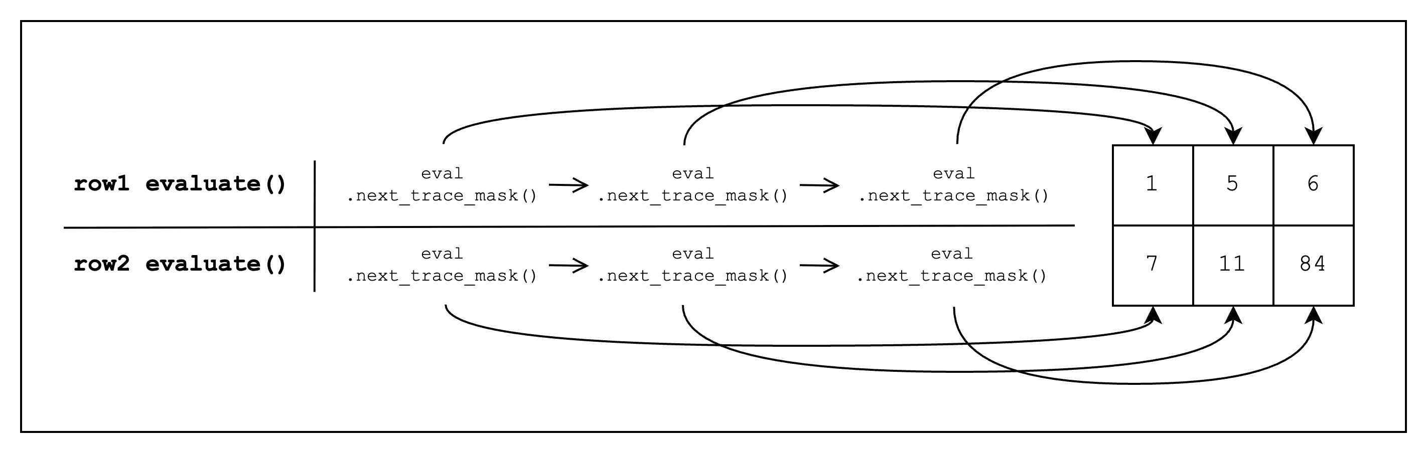
Inside FrameworkEval::evaluate, we call eval.next_trace_mask() consecutively three times, retrieving the cell values of all three columns (see Figure 3 below for a visual representation). Once we retrieve all three column values, we add a constraint of the form col_1 * col_2 + col_1 - col_3, which should equal 0.

We also need to implement FrameworkEval::max_constraint_log_degree_bound(&self) for FrameworkEval. As mentioned in the Composition Polynomial section, we need to expand the trace polynomial evaluations because the degree of our composition polynomial is higher than the trace polynomial. Expanding it by the lowest value CONSTRAINT_EVAL_BLOWUP_FACTOR=1 is sufficient for our example as the degree of our composition polynomial is not very high, so we can return self.log_size + CONSTRAINT_EVAL_BLOWUP_FACTOR. For those who are interested in how to set this value in general, we leave a detailed note below.

    // Precompute twiddles for evaluating and interpolating the trace
    let twiddles = SimdBackend::precompute_twiddles(
        CanonicCoset::new(
            log_num_rows + CONSTRAINT_EVAL_BLOWUP_FACTOR + config.fri_config.log_blowup_factor,
        )
        .circle_domain()
        .half_coset,
    );

Using the new TestEval struct, we can create a new FrameworkComponent::<TestEval> component, which the prover will use to evaluate the constraint. For now, we can ignore the other parameters of the FrameworkComponent::<TestEval> constructor.

We now move on to the final section where we finally create and verify a proof.