Introduction
Stwo is a state-of-the-art framework for creating STARK proofs that provides the following features:
- A frontend designed to be flexible to allow you to express your own constraints
- A backend that leverages Circle STARKs over the Mersenne31 prime field for fast prover performance
- Seamlessly integrated with Cairo
This book will guide you through the process of creating your own constraints and then proving them using Stwo. It will also provide in-depth explanations of the inner workings of how Stwo implements Circle STARKs.
Why Use a Proof System?
At its core, a proof system proves that a statement is valid. For example, it can prove that a function with a certain input results in a certain output, i.e. . To check the statement, we can do it either directly by computing and comparing the result to , or indirectly by verifying the proof. The verifier can benefit from the second option in terms of time and space, if the time to verify the proof is faster than the time to compute the function, or the size of the proof is smaller than the input to the statement.
This property of a proof system is often referred to as succinctness, and it is exactly why proof systems have seen wide adoption in the blockchain space, where computation on-chain is much more expensive compared to off-chain computation. Using a proof system, it becomes possible to replace a large collection of computation to be executed on-chain with a proof of execution of the same collection of computations and verifying it on-chain. This way, proofs can be generated off-chain using large machines and verified on-chain with much less computation.
But there are applications of proof systems beyond just blockchains. Generally speaking, it can be used as auxiliary data to verify that the computation of an untrusted party was done correctly. For example, when we delegate computation to an untrusted server, we can ask it to provide a proof along with the computation result that the result indeed came from running a specific computation. Another example could be to ask a server running an ML model to provide proof that it ran inference on the correct model. The size of the accompanying proof and the time to verify it will be negligible compared to the cost of running the computation, but we gain the guarantee that the computation was done correctly.
Another optional feature of proof systems is zero-knowledge, which means that the proof reveals nothing about the computation other than its validity. In general, the output of the computation will be public (i.e. revealed to the verifier), but the input will be, without loss of generality, private from the verifier. With this feature, the intermediate values computed by the prover while computing will also be hidden from the verifier.
Why Stwo?
Before we dive into why we should choose Stwo, let's define some terminology. When we talked about proof systems in the previous section, we mentioned that we can create a proof of a statement using a proof system. In reality, however, we first need to structure the function involved in the statement in a way that it can be proven. This structuring part is often referred to as the frontend, while the rest of the process of creating a proof is commonly referred to as the backend.
With that out of the way, let's dive into some of the advantages of using Stwo.
First, Stwo is a standalone framework that provides both the frontend and backend and therefore handles the entire proving process. There are other frameworks that only provide the frontend or the backend, which has its advantages as its modular structure makes it possible to pick and choose a backend or frontend of one's liking. However, having a single integrated frontend and backend reduces the complexity of the system and is also easier to maintain.
In addition, Stwo's frontend structures statements as an Algebraic Intermediate Representation (AIR), which is a representation that is especially useful for proving statements that are repetitive (e.g. the CPU in a VM, which essentially repeats the same fetch-decode-execute over and over again).
Stwo's backend is also optimized for prover performance. This is due to largely three factors.
-
It implements STARKs, or hash-based SNARKs, which boasts a faster prover compared to elliptic curve-based SNARKs like Groth16 or PLONK. This improvement comes mainly from running the majority of the computation in a small prime field (32 bits); Elliptic curve-based SNARKs, on the other hand, need to use big prime fields (e.g. 254-bit prime fields), which incur a lot of overhead as most computation does not require that many bits.
-
Even amongst multiple STARK backends, however, Stwo provides state-of-the-art prover performance by running the Mersenne-31 prime field (modulo ), which is faster than another popular 32-bit prime field like BabyBear (modulo ). We suggest going through this post for a breakdown of why this is the case.
-
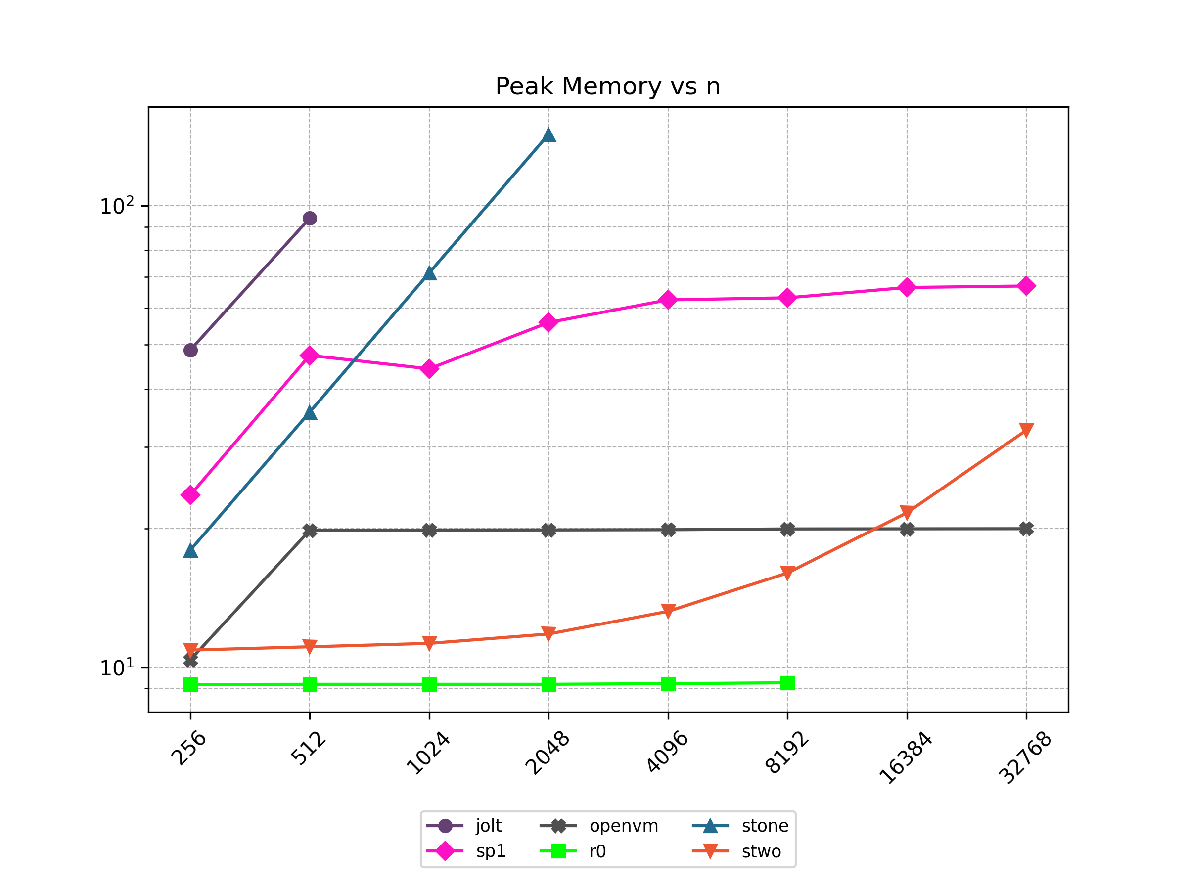
Finally, Stwo offers various CPU and GPU optimizations that improves prover performance as shown in Figure 1 below. It can also be compiled to WASM, allowing for fast proving in web environments.
One of the drawbacks of STARKs is that they have a larger proof size compared to elliptic curve-based SNARKs. One way to mitigate this drawback is by batching multiple proofs together to form a single proof.
On zero-knowledge:
As of the time of this writing, Stwo does not provide the "zero-knowledge" feature. "Zero-knowledge" here refers to the fact that the proof should not reveal any additional information other than the validity of the statement, which is not true for Stwo as it reveals to the verifier commitments to its witness values without hiding them by e.g. adding randomness. This reveals some information about the witness values, which may be used in conjunction with other information to infer the witness values.
AIR Development
This section is intended for developers who want to create custom proofs using Stwo (proofs of custom VMs, ML inference, etc.). It assumes that the reader is familiar with Rust and has some background knowledge of cryptography (e.g. finite fields). It also assumes that the reader is familiar with the concept of proof systems and knows what they want to create proofs for, but it does not assume any prior experience with creating them.
All the code that appears throughout this section is available here.
First Breath of AIR
Welcome to the guide for writing AIRs in Stwo!
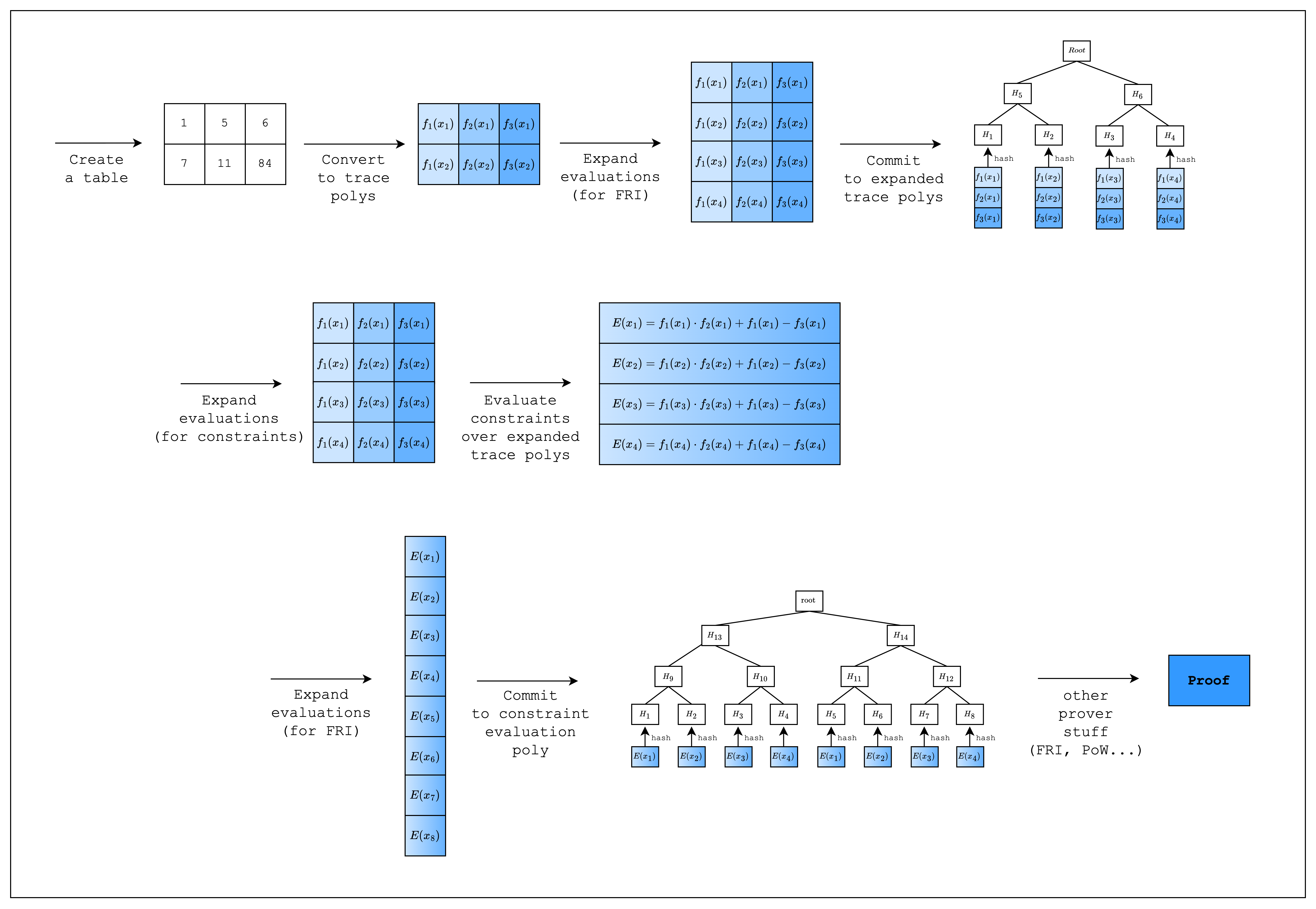
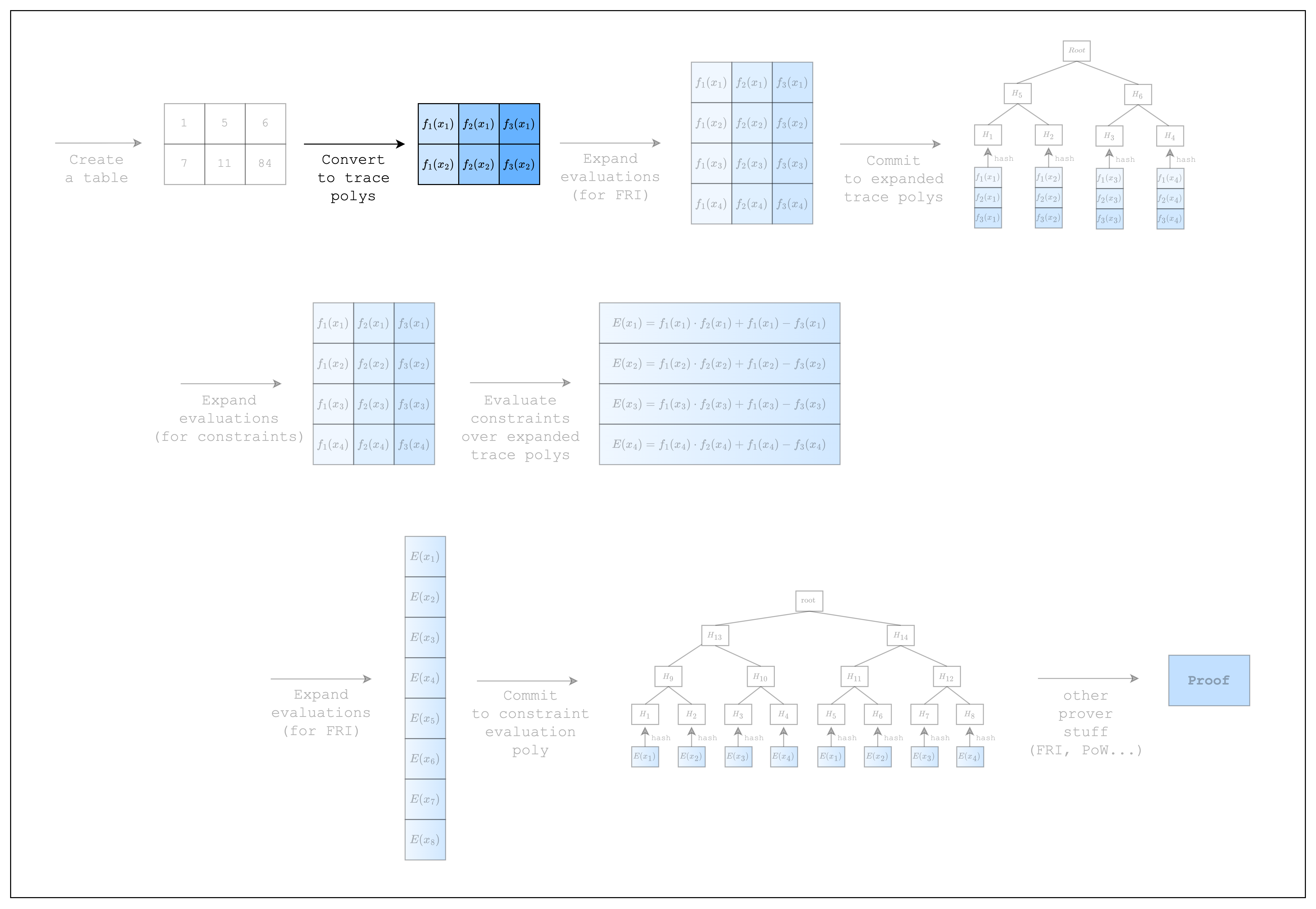
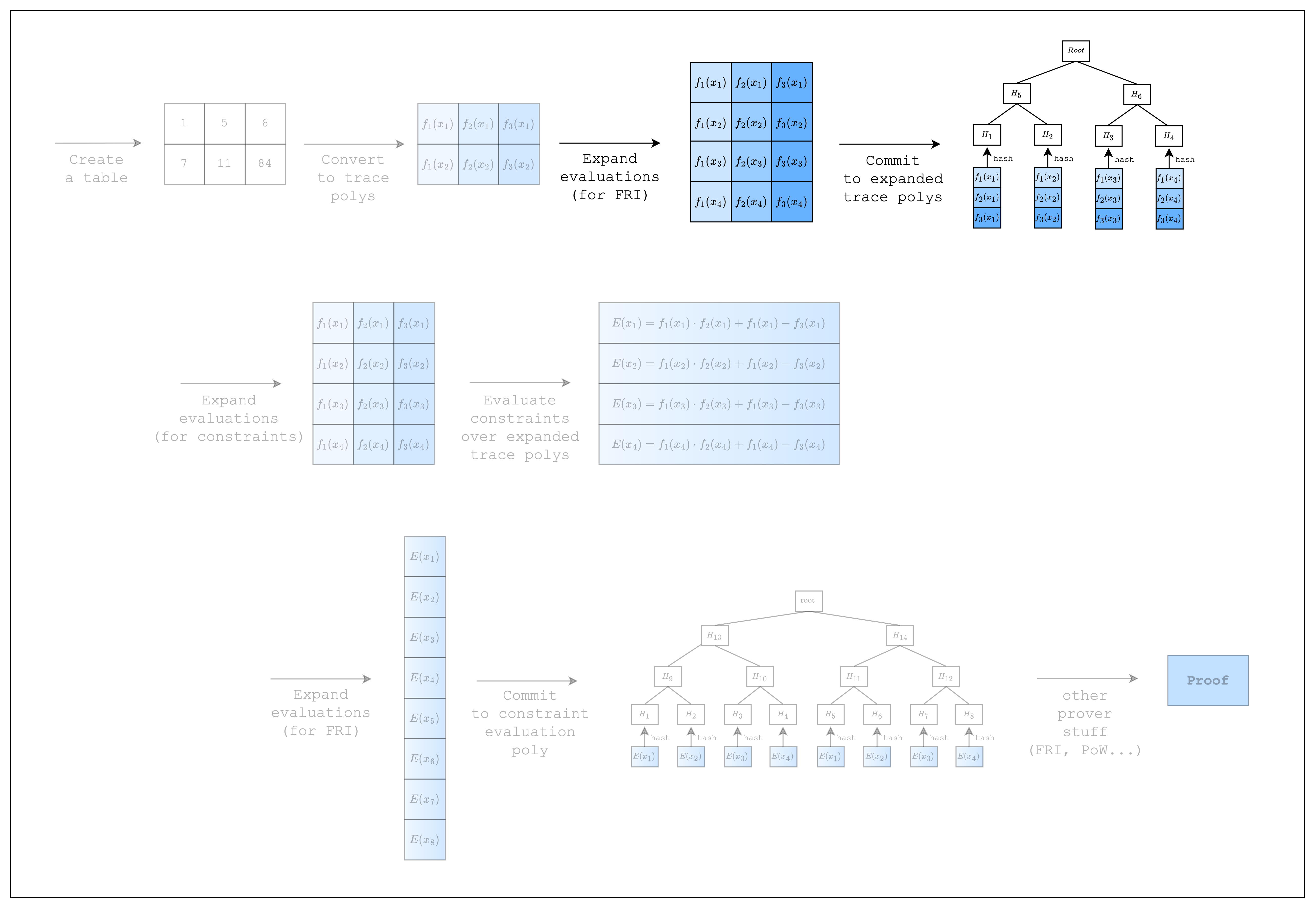
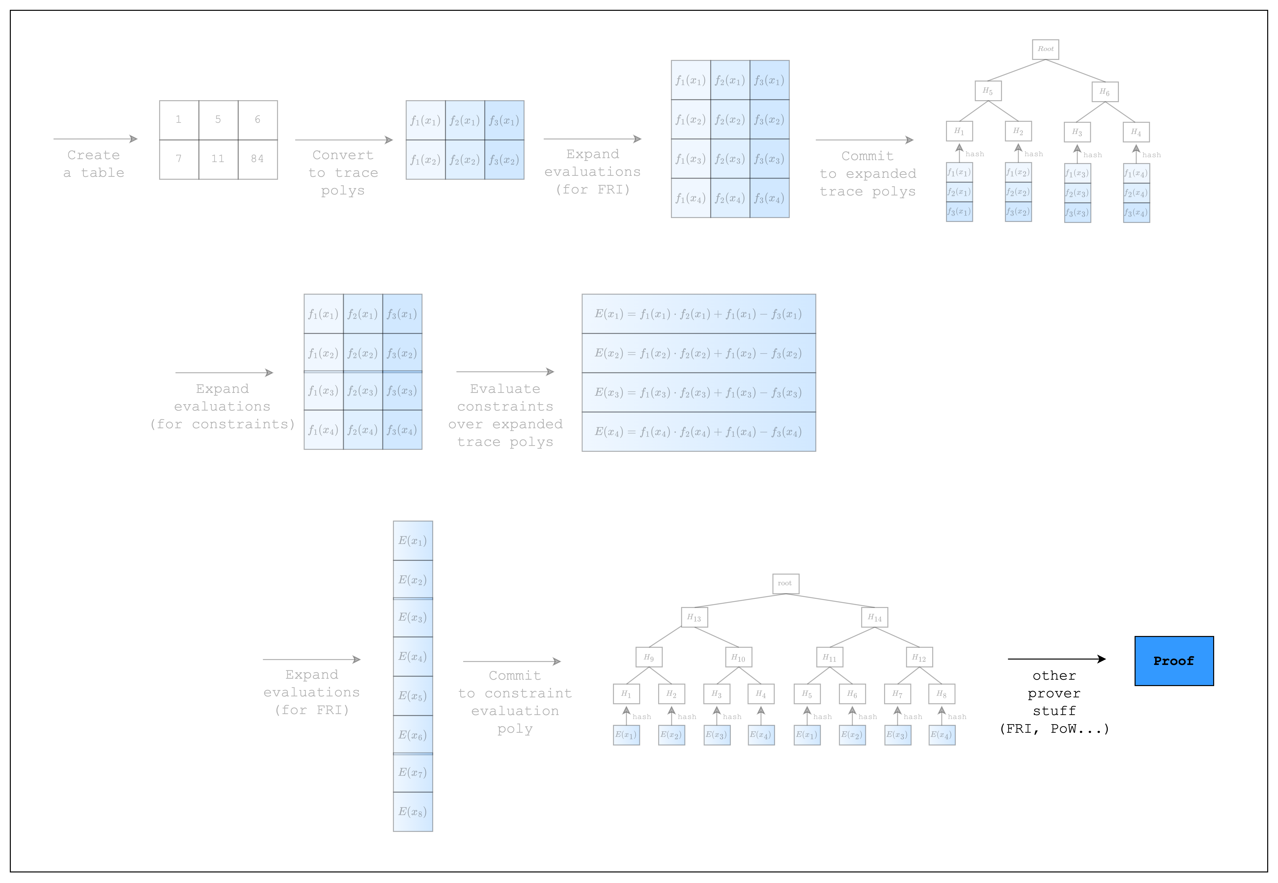
In this section, we will go through the process of writing a simple AIR from scratch. This requires some understanding of the proving lifecycle in Stwo, so we added a diagram showing a high-level overview of the whole process. As we go through each step, please note that the diagram may contain more steps than the code. This is because there are steps that are abstracted away by the Stwo implementation, but are necessary to understand the code that we write when creating an AIR.
Hello World
Let's first set up a Rust project with Stwo.
$ cargo new stwo-example
We need to specify the nightly Rust version to use Stwo.
$ echo -e "[toolchain]\nchannel = \"nightly-2025-01-02\"" > rust-toolchain.toml
Now let's edit the Cargo.toml file as follows:
[package]
name = "stwo-examples"
version = "0.1.0"
edition = "2021"
license = "MIT"

[dependencies]
stwo = { git = "https://github.com/starkware-libs/stwo.git", rev = "75a6b0ac9bcc7101d8658445dded51923ab2586f", features = ["prover"]}
stwo-constraint-framework = { git = "https://github.com/starkware-libs/stwo.git", rev = "75a6b0ac9bcc7101d8658445dded51923ab2586f", package = "stwo-constraint-framework", features = ["prover"] }
num-traits = "0.2.17"
itertools = "0.12.0"
rand = "0.8.5"
We are all set!
Writing a Spreadsheet
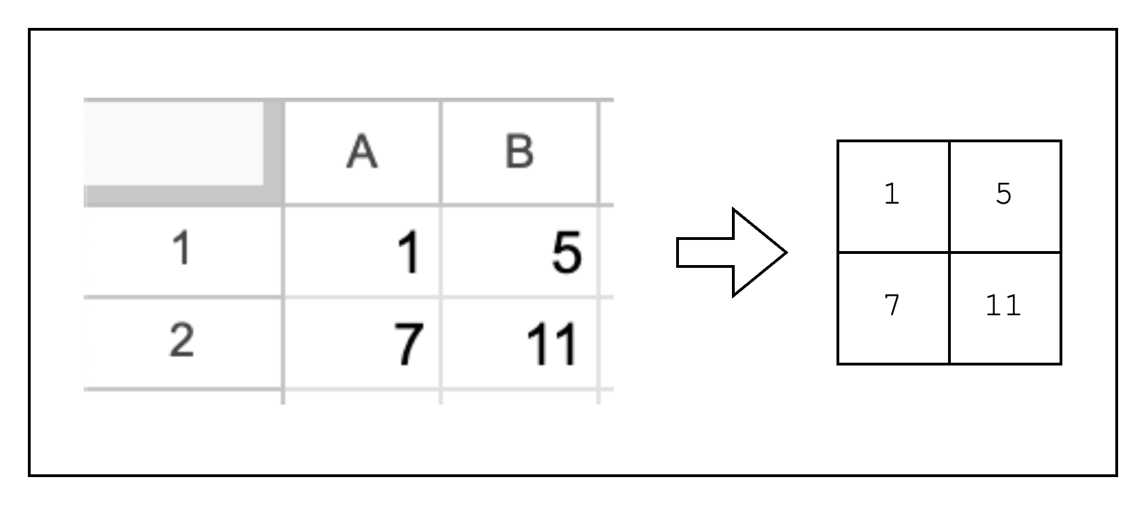
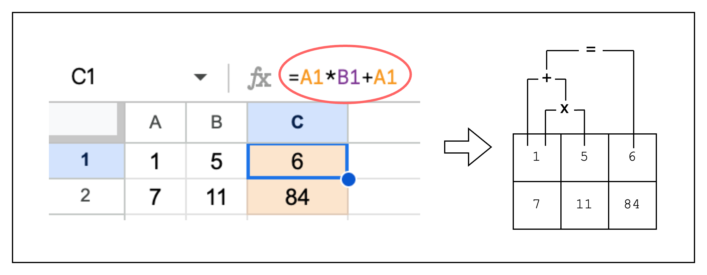
In order to write a proof, we first need to create a table of rows and columns. This is no different from writing integers to an Excel spreadsheet as we can see in Figure 2.
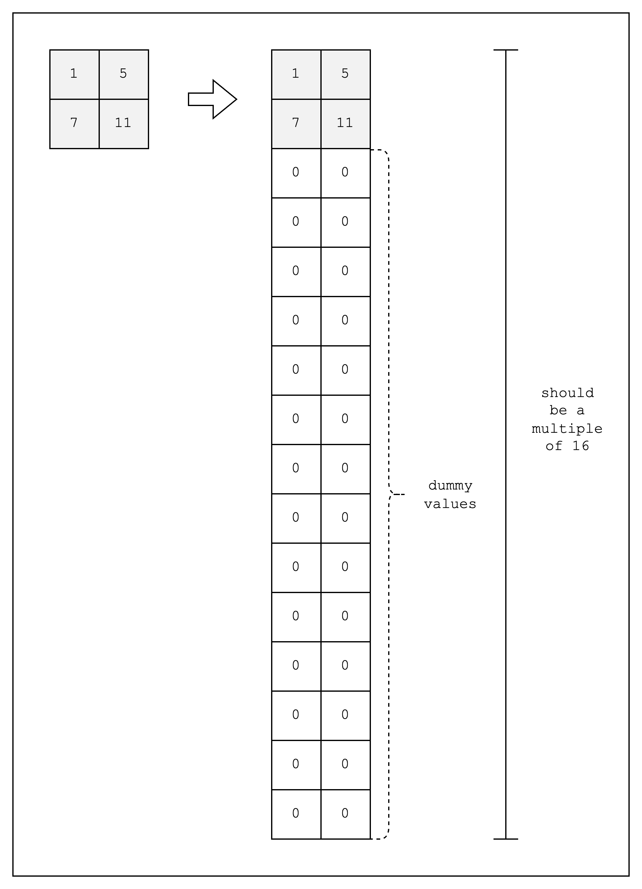
But there is a slight caveat to consider when creating the table. Stwo implements SIMD operations to speed up the prover in the CPU, but this requires providing the table cells in chunks of 16 rows. Simply put, this is because Stwo supports 16 lanes of 32-bit integers, which means that the same instruction can be run simultaneously for 16 different data.
Alas, for our table, we will need to create 14 dummy rows to make the total number of rows equal to 16, as shown in Figure 3. For the sake of simplicity, however, we will omit the dummy rows in the diagrams of the following sections.
Given all that, let's create this table using Stwo.
use stwo::prover::{
    backend::{
        simd::{column::BaseColumn, m31::N_LANES},
        Column,
    },
};
use stwo::core::fields::m31::M31;

fn main() {
    let num_rows = N_LANES;

    let mut col_1 = BaseColumn::zeros(num_rows as usize);
    col_1.set(0, M31::from(1));
    col_1.set(1, M31::from(7));

    let mut col_2 = BaseColumn::zeros(num_rows as usize);
    col_2.set(0, M31::from(5));
    col_2.set(1, M31::from(11));
}
As mentioned above, we instantiate the num_rows of our table as N_LANES=16 to accommodate SIMD operations. Then we create a BaseColumn of N_LANES=16 rows for each column and populate the first two rows with our values and the rest with dummy values.
Note that the values in the BaseColumn need to be of type M31, which refers to the Mersenne-31 prime field that Stwo uses. This means that the integers in the table must lie in the range .
Now that we have our table, let's move on!
From Spreadsheet to Trace Polynomials
In the previous section, we created a table (aka spreadsheet). In this section, we will convert the table into something called trace polynomials.
In STARKs, the computation trace is represented as evaluations of a polynomial over some domain. Typically this domain is a coset of a multiplicative subgroup. But since the multiplicative subgroup of M31 is not smooth, Stwo works over the circle group which is the subgroup of degree-2 extension of M31 (as explained in the Mersenne Primes and Circle Group sections). Thus the domain in Stwo is formed of points on the circle curve. Note that when we interpolate a polynomial over the points on the circle curve, we get a bivariate trace polynomial .
We will explain why using a polynomial representation is useful in the next section, but for now, let's see how we can create trace polynomials for our code. Note that we are building upon the code from the previous section, so there's not much new code here.
fn main() {
    // --snip--

    // Convert table to trace polynomials
    let domain = CanonicCoset::new(log_num_rows).circle_domain();
    let _trace: ColumnVec<CircleEvaluation<SimdBackend, M31, BitReversedOrder>> =
        vec![col_1, col_2]
            .into_iter()
            .map(|col| CircleEvaluation::new(domain, col))
            .collect();
}
Here, domain refers to the values used to interpolate the trace polynomials. For example, in Figure 2 are the domain values for our example. Note that when creating the domain, we set the log_num_rows to the log of the actual number of rows that are used in the table. In our example, we set it to 4 since Stwo requires that we use at least 16 rows. For a background on what CanonicCoset and .circle_domain() mean, you can refer to the Circle Group section.
Now that we have created 2 trace polynomials for our 2 columns, let's move on to the next section where we commit to those polynomials!
Committing to the Trace Polynomials
Now that we have created the trace polynomials, we need to commit to them.
As we can see in Figure 1, Stwo commits to the trace polynomials by first expanding the trace polynomials (i.e. adding more evaluations) and then committing to the expanded evaluations using a Merkle tree. The rate of expansion (commonly referred to as the blowup factor) is a parameter of the FRI protocol and for the purposes of this tutorial, we will use the default value.
const LOG_CONSTRAINT_EVAL_BLOWUP_FACTOR: u32 = 1;

fn main() {
    // --snip--

    // Config for FRI and PoW
    let config = PcsConfig::default();

    // Precompute twiddles for evaluating and interpolating the trace
    let twiddles = SimdBackend::precompute_twiddles(
        CanonicCoset::new(
            log_num_rows + LOG_CONSTRAINT_EVAL_BLOWUP_FACTOR + config.fri_config.log_blowup_factor,
        )
        .circle_domain()
        .half_coset,
    );

    // Create the channel and commitment scheme
    let channel = &mut Blake2sChannel::default();
    let mut commitment_scheme =
        CommitmentSchemeProver::<SimdBackend, Blake2sMerkleChannel>::new(config, &twiddles);

    // Commit to the preprocessed trace
    let mut tree_builder = commitment_scheme.tree_builder();
    tree_builder.extend_evals(vec![]);
    tree_builder.commit(channel);

    // Commit to the size of the trace
    channel.mix_u64(log_num_rows as u64);

    // Commit to the original trace
    let mut tree_builder = commitment_scheme.tree_builder();
    tree_builder.extend_evals(trace);
    tree_builder.commit(channel);
}
We begin with some setup. First, we create a default PcsConfig instance, which sets the values for the FRI and PoW operations. Setting non-default values is related to the security of the proof, which is outside the scope of this tutorial.
Next, we precompute twiddles, which are factors multiplied during FFT for a particular domain. Notice that the log size of the domain is set to log_num_rows + LOG_CONSTRAINT_EVAL_BLOWUP_FACTOR + config.fri_config.log_blowup_factor, which is the max log size of the domain that is needed throughout the proving process. For committing to the trace polynomial, we only need to add config.fri_config.log_blowup_factor but as we will see in the next section, we also need to commit to a polynomial of a higher degree, which is the reason we also add LOG_CONSTRAINT_EVAL_BLOWUP_FACTOR.
The final setup is creating a commitment scheme and a channel. The commitment scheme will be used to commit to the trace polynomials as Merkle trees, while the channel will be used to keep a running hash of all data in the proving process (i.e. transcript of the proof). This is part of the Fiat-Shamir transformation, which derives randomness safely in a non-interactive setting. Here, we use the Blake2sChannel and Blake2sMerkleChannel for the channel and commitment scheme, respectively, but we can also use the Poseidon252Channel and Poseidon252MerkleChannel pair.
Now that we have our setup, we can commit to the trace polynomials. But before we do so, we need to first commit to an empty vector called a preprocessed trace, which doesn't do anything but is required by Stwo. Then, we need to commit to the size of the trace, which is another vital part that the prover should not be able to cheat on. After doing so, we can finally commit to the original trace polynomials.
Now that we have committed to the trace polynomials, we can move on to how we can create constraints over the trace polynomials!
Evaluating Constraints Over Trace Polynomials
Proving Spreadsheet Functions
When we want to perform computations over the cells in a spreadsheet, we don't want to manually fill in the computed values. Instead, we leverage spreadsheet functions to autofill cells based on a given computation.
We can do the same thing with our table, except in addition to autofilling cells, we can also create a constraint that the result was computed correctly. Remember that the purpose of using a proof system is that the verifier can verify a computation was executed correctly without having to execute it themselves? Well, that's exactly why we need to create a constraint.
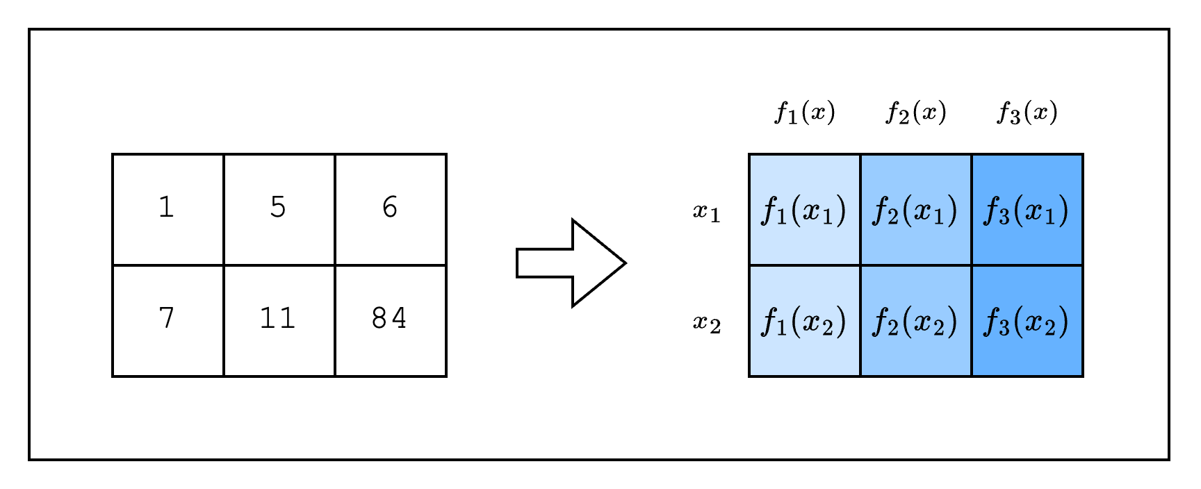
Now let's say we want to add a new column C to our spreadsheet that computes the product of the previous columns plus the first column. We can set C1 as A1 * B1 + A1 as in Figure 2. The corresponding constraint is expressed as C1 = A1 * B1 + A1. However, we use an alternate representation A1 * B1 + A1 - C1 = 0 because we can only enforce constraints stating that an expression should equal zero. Generalizing this constraint to the whole column, we get col1_row1 * col2_row1 + col1_row1 - col3_row1 = 0.
Identical Constraints Every Row
Obviously, as can be seen in Figure 2, our new constraint is satisfied for every row in the table. This means that we can substitute creating a constraint for each row with a single constraint over the columns, i.e. the trace polynomials.
Thus, col1_row1 * col2_row1 + col1_row1 - col3_row1 = 0 becomes:
The idea that all rows must have the same constraint may seem restrictive, compared to say a spreadsheet where we can define different functions for different rows. However, we will show in later sections how to handle such use-cases.
(Spoiler alert: it involves selectors and components)
Composition Polynomial
We will now give a name to the polynomial that expresses the constraint: a composition polynomial.
Basically, in order to prove that the constraints are satisfied, we need to show that the composition polynomial evaluates to 0 over the original domain (i.e. the domain of size the number of rows in the table).
But first, as can be seen in the upper part of Figure 1, we need to expand the evaluations of the trace polynomials by a factor of 2. This is because when you multiply two trace polynomials of degree n-1 (where n is the number of rows) to compute the constraint polynomial, the degree of the constraint polynomial will be the sum of the degrees of the trace polynomials, which is 2n-2. To adjust for this increase in degree, we double the number of evaluations.
Once we have the expanded evaluations, we can evaluate the composition polynomial . Since we need to do a FRI operation on the composition polynomial as well, we expand the evaluations again by a factor of 2 and commit to them as a merkle tree. This part corresponds to the bottom part of Figure 1.
Implementation
Let's see how this is implemented in the code.
struct TestEval {
    log_size: u32,
}

impl FrameworkEval for TestEval {
    fn log_size(&self) -> u32 {
        self.log_size
    }

    fn max_constraint_log_degree_bound(&self) -> u32 {
        self.log_size + LOG_CONSTRAINT_EVAL_BLOWUP_FACTOR
    }

    fn evaluate<E: EvalAtRow>(&self, mut eval: E) -> E {
        let col_1 = eval.next_trace_mask();
        let col_2 = eval.next_trace_mask();
        let col_3 = eval.next_trace_mask();
        eval.add_constraint(col_1.clone() * col_2.clone() + col_1.clone() - col_3.clone());
        eval
    }
}

fn main() {
    // --snip--

    let mut col_3 = BaseColumn::zeros(num_rows);
    col_3.set(0, col_1.at(0) * col_2.at(0) + col_1.at(0));
    col_3.set(1, col_1.at(1) * col_2.at(1) + col_1.at(1));

    // Convert table to trace polynomials
    let domain = CanonicCoset::new(log_num_rows).circle_domain();
    let trace: ColumnVec<CircleEvaluation<SimdBackend, M31, BitReversedOrder>> =
        vec![col_1, col_2, col_3]
            .into_iter()
            .map(|col| CircleEvaluation::new(domain, col))
            .collect();

    // --snip--

    // Create a component
    let _component = FrameworkComponent::<TestEval>::new(
        &mut TraceLocationAllocator::default(),
        TestEval {
            log_size: log_num_rows,
        },
        QM31::zero(),
    );
}
First, we add a new column col_3 that contains the result of the computation: col_1 * col_2 + col_1. Note that all the columns are padded with 0 to a length of 16 via BaseColumn::zeros(num_rows) and we got lucky because this satisfies our constraint (i.e. 0 * 0 + 0 - 0 = 0), so we don't need to modify the constraint.
Then, to create a constraint over the trace polynomials, we first create a TestEval struct that implements the FrameworkEval trait. Then, we add our constraint logic in the FrameworkEval::evaluate function. Note that this function is called for every row in the table, so we only need to define the constraint once.
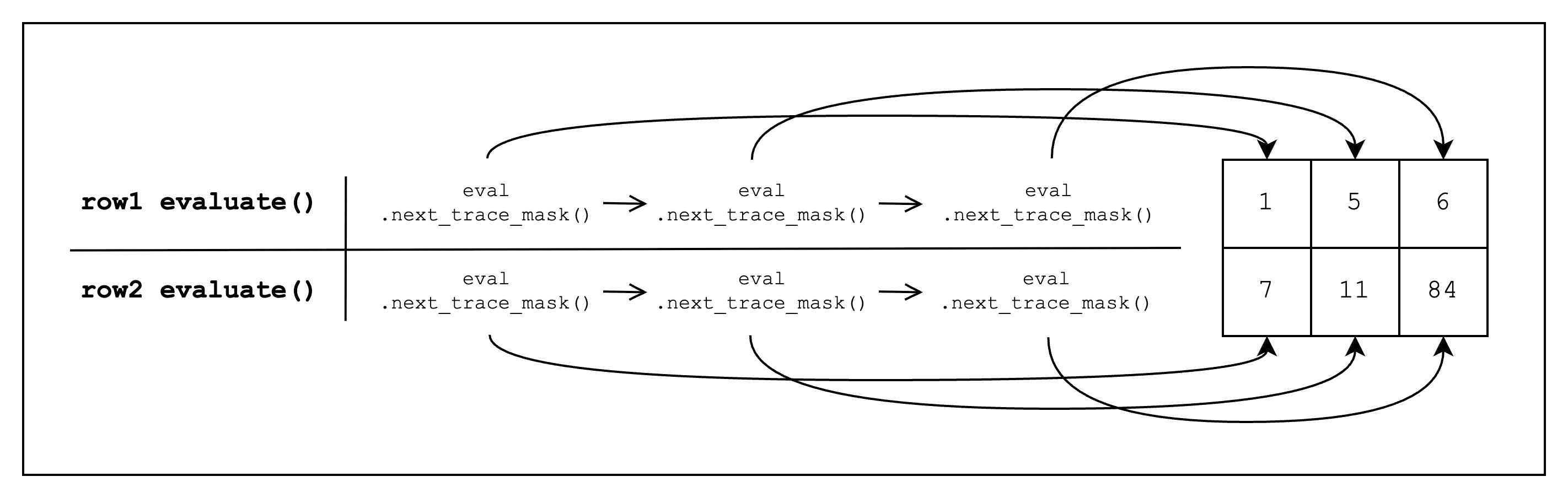
Inside FrameworkEval::evaluate, we call eval.next_trace_mask() consecutively three times, retrieving the cell values of all three columns (see Figure 3 below for a visual representation). Once we retrieve all three column values, we add a constraint of the form col_1 * col_2 + col_1 - col_3, which should equal 0. Note that FrameworkEval::evaluate will be called for every row in the table.
We also need to implement FrameworkEval::max_constraint_log_degree_bound(&self) for FrameworkEval. As mentioned in the Composition Polynomial section, we need to expand the trace polynomial evaluations because the degree of our composition polynomial is higher than that of the trace polynomial. Expanding it by LOG_CONSTRAINT_EVAL_BLOWUP_FACTOR=1 is sufficient for our example as the total degree of the highest degree term is 2, so we return self.log_size + LOG_CONSTRAINT_EVAL_BLOWUP_FACTOR. For those who are interested in how to set this value in general, we leave a detailed note below.
What value to set for max_constraint_log_degree_bound(&self)?
self.log_size + max(1, ceil(log2(max_degree - 1))), where max_degree is the maximum total degree of all defined constraint polynomials. For example, the max_degree of constraint is 2, while that of is 4.
e.g.
- degree 1 - 3:
self.log_size + 1 - degree 4 - 5:
self.log_size + 2 - degree 6 - 9:
self.log_size + 3 - degree 10 - 17:
self.log_size + 4 - ...
Now that we know the degree of the composition polynomial, we can see why we need to set the log_size of the domain to log_num_rows + LOG_CONSTRAINT_EVAL_BLOWUP_FACTOR + config.fri_config.log_blowup_factor when precomputing twiddles in the following code:
    // Precompute twiddles for evaluating and interpolating the trace
    let twiddles = SimdBackend::precompute_twiddles(
        CanonicCoset::new(
            log_num_rows + LOG_CONSTRAINT_EVAL_BLOWUP_FACTOR + config.fri_config.log_blowup_factor,
        )
        .circle_domain()
        .half_coset,
    );
To prove that the composition polynomial evaluates to 0 over the trace domain (since the composition polynomial is composed of constraints that evaluates to 0 over the trace domain), we first divide the composition polynomial by the vanishing polynomial, which is a polynomial that evaluates to 0 over the trace domain. If the composition polynomial is created correctly, this will result in a polynomial instead of a rational function, and we can perform FRI over this polynomial to prove this.
Thus, we need to commit to this new polynomial, which is called the quotient polynomial. We can calculate its degree by subtracting the degree of the vanishing polynomial from the degree of the composition polynomial. Since the trace is of size 1 << log_num_rows, the degree of the vanishing polynomial will be 1 << log_num_rows - 1, so the resulting degree will be 1 << (log_num_rows + LOG_CONSTRAINT_EVAL_BLOWUP_FACTOR) - (1 << log_num_rows - 1). However, since we can only commit to a power of two degree, we can just use the 1 << (log_num_rows + LOG_CONSTRAINT_EVAL_BLOWUP_FACTOR) value.
If we apply the FRI blowup as well, we finally end up with the following log domain size: log_num_rows + LOG_CONSTRAINT_EVAL_BLOWUP_FACTOR + config.fri_config.log_blowup_factor.
Using the new TestEval struct, we can create a new FrameworkComponent::<TestEval> component, which the prover will use to evaluate the constraint. For now, we can ignore the other parameters of the FrameworkComponent::<TestEval> constructor.
We now move on to the final section where we finally create and verify a proof.
Finally, we can break down what an Algebraic Intermediate Representation (AIR) means.
Algebraic means that we are using polynomials to represent the constraints.
Intermediate Representation means that this is a modified representation of our statement so that it can be proven.
So AIR is just another way of saying that we are representing statements to be proven as constraints over polynomials.
Proving and Verifying an AIR
We're finally ready for the last step: prove and verify an AIR!
Since the code is relatively short, let us present it first and then go over the details.
fn main() {
    // --snip--

    // Prove
    let proof = prove(&[&component], channel, commitment_scheme).unwrap();

    // Verify
    let channel = &mut Blake2sChannel::default();
    let commitment_scheme = &mut CommitmentSchemeVerifier::<Blake2sMerkleChannel>::new(config);
    let sizes = component.trace_log_degree_bounds();

    commitment_scheme.commit(proof.commitments[0], &sizes[0], channel);
    channel.mix_u64(log_num_rows as u64);
    commitment_scheme.commit(proof.commitments[1], &sizes[1], channel);

    verify(&[&component], channel, commitment_scheme, proof).unwrap();
}
Prove
As you can see, there is only a single line of code added to create the proof. The prove function performs the FRI and PoW operations under the hood, although, technically, the constraint-related steps in Figure 1 were not performed in the previous section and are only performed once prove is called.
Verify
In order to verify our proof, we need to check that the constraints are satisfied using the commitments from the proof. In order to do that, we need to set up a Blake2sChannel and CommitmentSchemeVerifier<Blake2sMerkleChannel>, along with the same PcsConfig that we used when creating the proof. Then, we need to recreate the Fiat-Shamir channel by passing the Merkle tree commitments and the log_num_rows to the CommitmentSchemeVerifier instance by calling commit (remember: the order is important!). Then, we can verify the proof using the verify function.
Try setting the dummy values in the table to 1 instead of 0. Does it fail? If so, can you see why?
Congratulations! We have come full circle. We now know how to create a table, convert it to trace polynomials, commit to them, create constraints over the trace polynomials, and prove and verify the constraints (i.e. an AIR). In the following sections, we will go over some more complicated AIRs to explain Stwo's other features.
Preprocessed Trace
This section and the following sections are intended for developers who have completed the First Breath of AIR section or are already familiar with the workflow of creating an AIR. If you have not gone through the previous section, we recommend doing so first as the following sections gloss over a lot of boilerplate code.
For those of you who have completed the First Breath of AIR tutorial, you should now be familiar with the concept of a trace as a table of integers that are filled in by the prover (we will now refer to this as the original trace).
In addition to the original trace, Stwo also has a concept of a preprocessed trace, which is a table whose values are fixed and therefore cannot be arbitrarily chosen by the prover. In other words, these are columns whose values are known in advance of creating a proof and essentially agreed upon by both the prover and the verifier.
One of the use cases of the preprocessed trace is as a selector for different constraints. Remember that in an AIR, the same constraints are applied to every row of the trace? If we go back to the spreadsheet analogy, this means that we can't create a spreadsheet that runs different computations for different rows. To get around this, note that if we multiply a constraint with a "selector" that is zero, the constraint will be trivially satisfied. Building on this, we can create a selector column of 0s and 1s, and multiply the constraint with the selector column. For example, let's say we want to create a constraint that runs different computations for the first 2 rows and the next 2 rows. We can do this by creating a selector column that has value 0 for the first 2 rows and 1 for the next 2 rows and combining it with the constraints as follows:
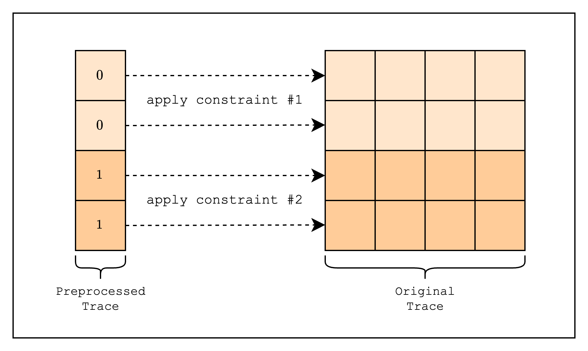
Another use case is to use the preprocessed trace to express constant values used in constraints. For example, when creating a hash function in an AIR, we often need to use round constants, which the verifier needs to be able to verify or the resulting hash may be invalid. We can also "look up" the constant values as an optimization technique, which we will discuss in more detail in the next section.
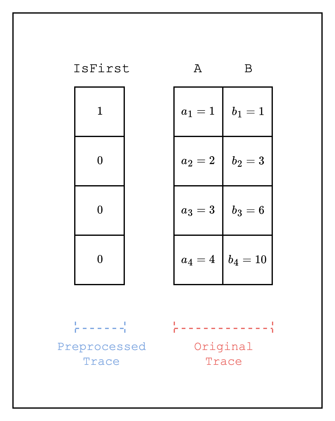
In this section, we will explore how to implement a preprocessed trace as a selector, and we will implement the simplest form: a single IsFirst column, where the value is 1 for the first row and 0 for all other rows.
Boilerplate code is omitted for brevity. Please refer to the full example code for the full implementation.
struct IsFirstColumn {
    pub log_size: u32,
}

#[allow(dead_code)]
impl IsFirstColumn {
    pub fn new(log_size: u32) -> Self {
        Self { log_size }
    }

    pub fn gen_column(&self) -> CircleEvaluation<SimdBackend, M31, BitReversedOrder> {
        let mut col = BaseColumn::zeros(1 << self.log_size);
        col.set(0, M31::from(1));
        CircleEvaluation::new(CanonicCoset::new(self.log_size).circle_domain(), col)
    }

    pub fn id(&self) -> PreProcessedColumnId {
        PreProcessedColumnId {
            id: format!("is_first_{}", self.log_size),
        }
    }
}
First, we need to define an IsFirstColumn struct that will be used as a preprocessed trace. We will use the gen_column() function to generate a CircleEvaluation struct that is 1 for the first row and 0 for all other rows. The id() function is needed to identify this column when evaluating the constraints.
fn main() {
    ...
    // Create and commit to the preprocessed trace
    let is_first_column = IsFirstColumn::new(log_size);
    let mut tree_builder = commitment_scheme.tree_builder();
    tree_builder.extend_evals(vec![is_first_column.gen_column()]);
    tree_builder.commit(channel);

    // Commit to the size of the trace
    channel.mix_u64(log_size as u64);

    // Create and commit to the original trace
    let trace = gen_trace(log_size);
    let mut tree_builder = commitment_scheme.tree_builder();
    tree_builder.extend_evals(trace);
    tree_builder.commit(channel);
    ...
}
Then, in our main function, we will create and commit to the preprocessed and original traces. For those of you who are curious about why we need to commit to the trace, please refer to the Committing to the Trace Polynomials section.
struct TestEval {
    is_first_id: PreProcessedColumnId,
    log_size: u32,
}

impl FrameworkEval for TestEval {
    fn log_size(&self) -> u32 {
        self.log_size
    }

    fn max_constraint_log_degree_bound(&self) -> u32 {
        self.log_size + LOG_CONSTRAINT_EVAL_BLOWUP_FACTOR
    }

    fn evaluate<E: EvalAtRow>(&self, mut eval: E) -> E {
        let is_first = eval.get_preprocessed_column(self.is_first_id.clone());

        let col_1 = eval.next_trace_mask();
        let col_2 = eval.next_trace_mask();
        let col_3 = eval.next_trace_mask();

        // If is_first is 1, then the constraint is col_1 * col_2 - col_3 = 0
        // If is_first is 0, then the constraint is col_1 * col_2 + col_1 - col_3 = 0
        eval.add_constraint(
            is_first.clone() * (col_1.clone() * col_2.clone() - col_3.clone())
                + (E::F::from(M31::from(1)) - is_first.clone())
                    * (col_1.clone() * col_2.clone() + col_1.clone() - col_3.clone()),
        );

        eval
    }
}
Now that we have the traces, we need to create a struct that contains the logic for evaluating the constraints. As mentioned before, we need to use the is_first_id field to retrieve the row value of the IsFirstColumn struct. Then, we compose two constraints using the IsFirstColumn row value as a selector and adding them together.
If you're unfamiliar with how max_constraint_log_degree_bound(&self) should be implemented, please refer to this note.
fn main() {
    ...
    // Create a component
    let component = FrameworkComponent::<TestEval>::new(
        &mut TraceLocationAllocator::default(),
        TestEval {
            is_first_id: is_first_column.id(),
            log_size,
        },
        QM31::zero(),
    );

    // Prove
    let proof = prove(&[&component], channel, commitment_scheme).unwrap();

    // Verify
    let channel = &mut Blake2sChannel::default();
    let commitment_scheme = &mut CommitmentSchemeVerifier::<Blake2sMerkleChannel>::new(config);
    let sizes = component.trace_log_degree_bounds();

    commitment_scheme.commit(proof.commitments[0], &sizes[0], channel);
    channel.mix_u64(log_size as u64);
    commitment_scheme.commit(proof.commitments[1], &sizes[1], channel);

    verify(&[&component], channel, commitment_scheme, proof).unwrap();
}
Finally, we can create a FrameworkComponent using the TestEval struct and then prove and verify the component.
Static Lookups
In the previous section, we showed how to create a preprocessed trace. In this section, we will introduce the concept of an interaction trace, and use it with the preprocessed trace to implement static lookups.
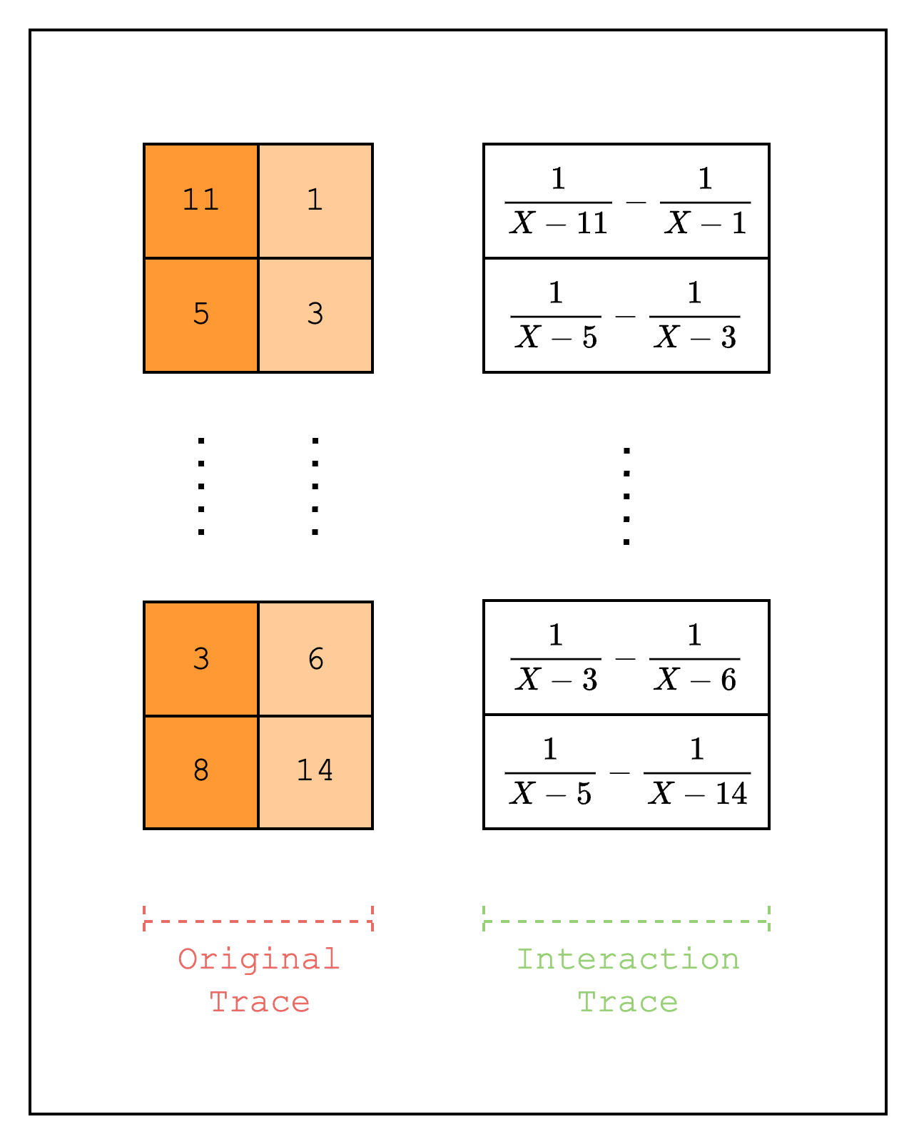
Let's start with a brief introduction to lookups. A lookup is a way to connect values from one part of the table to another part of the table. A simple example is when we want to copy values across parts of the table. At first glance, this seems feasible using a constraint. For example, we can copy values to by creating a constraint that is equal to . The limitation with this approach, however, is that the same constraint needs to be satisfied over every row in the columns. In other words, we can only check that is an exact copy of :
But what if we want to check that is a copy of regardless of the order of the values? This can be done by comparing that the grand product of the random linear combinations of all values in is equal to the grand product of the random linear combinations of all values in :
where is a random value from the verifier.
By taking the logarithmic derivative of each side of the equation, we can rewrite it:
We can go further and allow each of the original values to be copied a different number of times. This is supported by modifying the check to the following:
Where represents the multiplicity, or the number of times appears in .
In Stwo, these fractions (which we will hereafter refer to as LogUp fractions) are stored in a special type of trace called an interaction trace. An interaction trace is used to contain values that involve interaction between the prover and the verifier. As mentioned above, a LogUp fraction requires a random value from the verifier, which is why it is stored in an interaction trace.
Range-check AIR
We will now walk through the implementation of a static lookup, which is a lookup where the values that are being looked up are static, i.e. part of the preprocessed trace. Specifically, we will implement a range-check AIR, which checks that a certain value is within a given range. This is especially useful for frameworks like Stwo that use finite fields because it allows checking for underflow and overflow.
A range-check checks that all values in a column are within a certain range. For example, as in Figure 1, we can check that all values in the range-checked columns are between 0 and 3. We do this by first creating a multiplicity column that counts the number of times each value in the preprocessed trace appears in the range-checked columns.
Then, we create two LogUp columns as part of the interaction trace. The first column contains in each row a fraction with numerator equal to the multiplicity and denominator equal to the random linear combination of the value in the range column. For example, for row 1, the fraction should be , where is a random value. The second column contains batches of fractions where the denominator of each fraction is the random linear combination of the value in the range-checked column. Note that the numerator of each fraction is always -1, i.e. we apply a negation, because we want the sum of the first column to be equal to the sum of the second column.
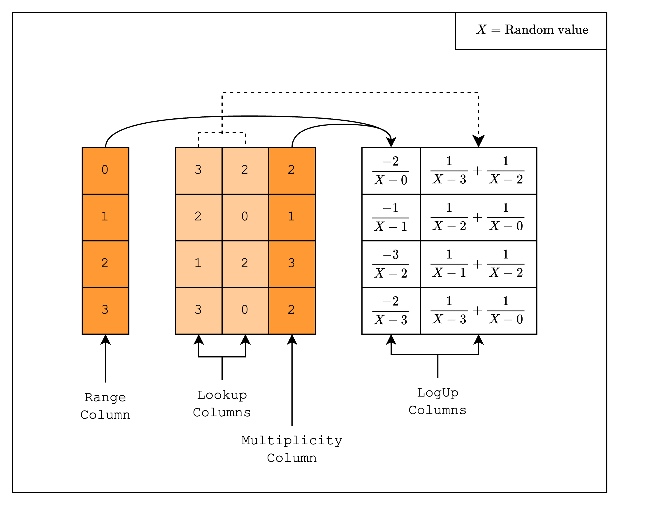
If we add all the fractions in the two columns together, we get 0. This means that the verifier will be convinced with high probability that the values in the range-checked columns are a subset of the values in the range column.
Implementation
Now let's move on to the implementation where we create a 4-bit range-check AIR. We do this by creating a preprocessed trace column with the integers , then using a lookup to force the values in the original trace columns to lie in the values of the preprocessed column.
struct RangeCheckColumn {
    pub log_size: u32,
}

#[allow(dead_code)]
impl RangeCheckColumn {
    pub fn new(log_size: u32) -> Self {
        Self { log_size }
    }

    pub fn gen_column(&self) -> CircleEvaluation<SimdBackend, M31, BitReversedOrder> {
        let col = BaseColumn::from_iter((0..(1 << self.log_size)).map(|i| M31::from(i)));
        CircleEvaluation::new(CanonicCoset::new(self.log_size).circle_domain(), col)
    }

    pub fn id(&self) -> PreProcessedColumnId {
        PreProcessedColumnId {
            id: format!("range_check_{}_bits", self.log_size),
        }
    }
}
First, we need to create the range-check column as a preprocessed column. This should look familiar to the code from the previous section.
fn gen_trace(log_size: u32) -> Vec<CircleEvaluation<SimdBackend, M31, BitReversedOrder>> {
    // Create a table with random values
    let mut rng = rand::thread_rng();
    let lookup_col_1 =
        BaseColumn::from_iter((0..(1 << log_size)).map(|_| M31::from(rng.gen_range(0..16))));
    let lookup_col_2 =
        BaseColumn::from_iter((0..(1 << log_size)).map(|_| M31::from(rng.gen_range(0..16))));

    let mut multiplicity_col = BaseColumn::zeros(1 << log_size);
    lookup_col_1
        .as_slice()
        .iter()
        .chain(lookup_col_2.as_slice().iter())
        .for_each(|value| {
            let index = value.0 as usize;
            multiplicity_col.set(index, multiplicity_col.at(index) + M31::from(1));
        });

    // Convert table to trace polynomials
    let domain = CanonicCoset::new(log_size).circle_domain();
    vec![
        lookup_col_1.clone(),
        lookup_col_2.clone(),
        multiplicity_col.clone(),
    ]
    .into_iter()
    .map(|col| CircleEvaluation::new(domain, col))
    .collect()
}
Next, we create the original trace columns. The first two columns are random values in the range , and the third column contains the counts of the values in the range-check column.
relation!(SmallerThan16Elements, 1);

fn gen_logup_trace(
    range_log_size: u32,
    log_size: u32,
    range_check_col: &BaseColumn,
    lookup_col_1: &BaseColumn,
    lookup_col_2: &BaseColumn,
    multiplicity_col: &BaseColumn,
    lookup_elements: &SmallerThan16Elements,
) -> (
    Vec<CircleEvaluation<SimdBackend, M31, BitReversedOrder>>,
    SecureField,
) {
    let mut logup_gen = LogupTraceGenerator::new(range_log_size);

    let mut col_gen = logup_gen.new_col();
    for simd_row in 0..(1 << (range_log_size - LOG_N_LANES)) {
        let numerator: PackedSecureField = PackedSecureField::from(multiplicity_col.data[simd_row]);
        let denom: PackedSecureField = lookup_elements.combine(&[range_check_col.data[simd_row]]);
        col_gen.write_frac(simd_row, -numerator, denom);
    }
    col_gen.finalize_col();

    let mut col_gen = logup_gen.new_col();
    for simd_row in 0..(1 << (log_size - LOG_N_LANES)) {
        let lookup_col_1_val: PackedSecureField =
            lookup_elements.combine(&[lookup_col_1.data[simd_row]]);
        let lookup_col_2_val: PackedSecureField =
            lookup_elements.combine(&[lookup_col_2.data[simd_row]]);
        // 1 / denom1 + 1 / denom2 = (denom1 + denom2) / (denom1 * denom2)
        let numerator = lookup_col_1_val + lookup_col_2_val;
        let denom = lookup_col_1_val * lookup_col_2_val;
        col_gen.write_frac(simd_row, numerator, denom);
    }
    col_gen.finalize_col();

    logup_gen.finalize_last()
}

fn main() {
    ...
    // Draw random elements to use when creating the random linear combination of lookup values in the LogUp columns
    let lookup_elements = SmallerThan16Elements::draw(channel);

    // Create and commit to the LogUp columns
    let (logup_cols, claimed_sum) = gen_logup_trace(
        range_log_size,
        log_num_rows,
        &range_check_col,
        &trace[0],
        &trace[1],
        &trace[2],
        &lookup_elements,
    );
    ...
}
Now we need to create the LogUp columns.
First, note that we are creating a SmallerThan16Elements instance using the macro relation!. This macro creates an API for performing random linear combinations. Under the hood, it creates two random values that can create a random linear combination of an arbitrary number of elements. In our case, we only need to combine one value (value in ), which is why we pass in 1 to the macro.
Inside gen_logup_trace, we create a LogupTraceGenerator instance. This is a helper class that allows us to create LogUp columns. Every time we create a new column, we need to call new_col() on the LogupTraceGenerator instance.
You may notice that we are iterating over BaseColumn in chunks of 16, or 1 << LOG_N_LANES values. This is because we are using the SimdBackend, which runs 16 lanes simultaneously, so we need to preserve this structure. The Packed in PackedSecureField means that it packs 16 values into a single value.
You may also notice that we are using a SecureField instead of just the Field. This is because the random value we created by SmallerThan16Elements lies in the degree-4 extension field . This is necessary for the security of the protocol and interested readers can refer to the Mersenne Primes section for more details.
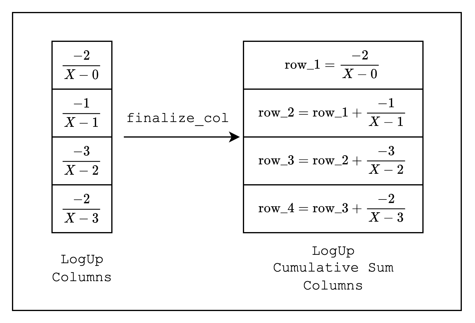
Once we set the fractions for each simd_row, we need to call finalize_col() to finalize the column. This process modifies the LogUp columns from individual fractions to cumulative sums of the fractions as shown in Figure 2.
Finally, we need to call finalize_last() on the LogupTraceGenerator instance to finalize the LogUp columns, which will return the LogUp columns as well as the sum of the fractions in the LogUp columns.
struct TestEval {
    range_check_id: PreProcessedColumnId,
    log_size: u32,
    lookup_elements: SmallerThan16Elements,
}

impl FrameworkEval for TestEval {
    fn log_size(&self) -> u32 {
        self.log_size
    }

    fn max_constraint_log_degree_bound(&self) -> u32 {
        self.log_size + LOG_CONSTRAINT_EVAL_BLOWUP_FACTOR
    }

    fn evaluate<E: EvalAtRow>(&self, mut eval: E) -> E {
        let range_check_col = eval.get_preprocessed_column(self.range_check_id.clone());

        let lookup_col_1 = eval.next_trace_mask();
        let lookup_col_2 = eval.next_trace_mask();
        let multiplicity_col = eval.next_trace_mask();

        eval.add_to_relation(RelationEntry::new(
            &self.lookup_elements,
            -E::EF::from(multiplicity_col),
            &[range_check_col],
        ));

        eval.add_to_relation(RelationEntry::new(
            &self.lookup_elements,
            E::EF::one(),
            &[lookup_col_1],
        ));

        eval.add_to_relation(RelationEntry::new(
            &self.lookup_elements,
            E::EF::one(),
            &[lookup_col_2],
        ));

        eval.finalize_logup_batched(&vec![0, 1, 1]);

        eval
    }
}
The last piece of the puzzle is to create the constraints. We use the same TestEval struct as in the previous sections, but the evaluate function will look slightly different. Instead of calling add_constraint on the EvalAtRow instance, we will call add_to_relation, which recreates the fractions that we added in the LogUp columns using values in the range-check, lookup, and multiplicity columns.
Once we add the fractions as constraints, we call the finalize_logup_batched function, which indicates how we want to batch the fractions. In our case, we added 3 fractions but want to create batches where the last two fractions are batched together, so we pass in &vec![0, 1, 1].
    // Verify
    assert_eq!(claimed_sum, SecureField::zero());

    let channel = &mut Blake2sChannel::default();
    let commitment_scheme = &mut CommitmentSchemeVerifier::<Blake2sMerkleChannel>::new(config);
    let sizes = component.trace_log_degree_bounds();

    commitment_scheme.commit(proof.commitments[0], &sizes[0], channel);
    channel.mix_u64((log_num_rows) as u64);
    commitment_scheme.commit(proof.commitments[1], &sizes[1], channel);
    commitment_scheme.commit(proof.commitments[2], &sizes[2], channel);

    verify(&[&component], channel, commitment_scheme, proof).unwrap();
When we verify the proof, as promised, we check that the claimed_sum, which is the sum of the fractions in the LogUp columns, is 0.
And that's it! We have successfully created a static lookup for a range-check.
How many fractions can we batch together?
This depends on how we set the max_constraint_log_degree_bound function, as discussed in this note. More specifically, we can batch up to exactly the blowup factor.
e.g.
self.log_size + 1-> 2 fractionsself.log_size + 2-> 4 fractionsself.log_size + 3-> 8 fractionsself.log_size + 4-> 16 fractions- ...
Note that unlike what Figure 1 shows, the size of the range column and the range-checked columns do not have to be the same. As we will learn in the Components section, we can create separate components for the range-check and the range-checked columns to support such cases.
Dynamic Lookups
In the last section, we implemented a static lookup. A dynamic lookup is the same as a static lookup except that the values that are being looked up are not known before the proving process (i.e. they are not preprocessed columns but trace columns).
In this section, we will implement one of the simplest dynamic lookups: a permutation check.
A permutation check simply checks that two sets of values have the same elements, but not necessarily in the same order. For example, the values and are a permutation of each other, but and are not.
If you went through the previous section, you should have a good intuition for how to implement this. First, create two original trace columns that each contain a random permutation of the same set of values. Then, create a LogUp column where the first original trace column is added as a fraction with multiplicity and the second original trace column is added as a fraction with multiplicity . Then, check that the claimed_sum, or the sum of the fractions in the two LogUp columns, is .
Let's move on to the implementation.
fn gen_trace(log_size: u32) -> Vec<CircleEvaluation<SimdBackend, M31, BitReversedOrder>> {
    let mut rng = rand::thread_rng();
    let values = (0..(1 << log_size)).map(|i| i).collect::<Vec<_>>();

    // Create a random permutation of the values
    let mut random_values = values.clone();
    random_values.shuffle(&mut rng);
    let random_col_1 = BaseColumn::from_iter(random_values.iter().map(|v| M31::from(*v)));

    // Create another random permutation of the values
    let mut random_values = random_values.clone();
    random_values.shuffle(&mut rng);
    let random_col_2 = BaseColumn::from_iter(random_values.iter().map(|v| M31::from(*v)));

    // Convert table to trace polynomials
    let domain = CanonicCoset::new(log_size).circle_domain();
    vec![random_col_1, random_col_2]
        .into_iter()
        .map(|col| CircleEvaluation::new(domain, col))
        .collect()
}

fn gen_logup_trace(
    log_size: u32,
    random_col_1: &BaseColumn,
    random_col_2: &BaseColumn,
    lookup_elements: &LookupElements,
) -> (
    Vec<CircleEvaluation<SimdBackend, M31, BitReversedOrder>>,
    SecureField,
) {
    let mut logup_gen = LogupTraceGenerator::new(log_size);

    let mut col_gen = logup_gen.new_col();
    for row in 0..(1 << (log_size - LOG_N_LANES)) {
        // 1 / random - 1 / ordered = (ordered - random) / (random * ordered)
        let random_val: PackedSecureField = lookup_elements.combine(&[random_col_1.data[row]]);
        let ordered_val: PackedSecureField = lookup_elements.combine(&[random_col_2.data[row]]);
        col_gen.write_frac(row, ordered_val - random_val, random_val * ordered_val);
    }
    col_gen.finalize_col();

    logup_gen.finalize_last()
}

fn main() {
    ...
    // Create and commit to the trace columns
    let trace = gen_trace(log_size);
    let mut tree_builder = commitment_scheme.tree_builder();
    tree_builder.extend_evals(trace.clone());
    tree_builder.commit(channel);

    // Draw random elements to use when creating the random linear combination of lookup values in the LogUp columns
    let lookup_elements = LookupElements::draw(channel);

    // Create and commit to the LogUp columns
    let (logup_cols, claimed_sum) =
        gen_logup_trace(log_size, &trace[0], &trace[1], &lookup_elements);
    let mut tree_builder = commitment_scheme.tree_builder();
    tree_builder.extend_evals(logup_cols);
    tree_builder.commit(channel);
    ...
}
Looking at the code above, we can see that it looks very similar to the implementation in the previous section. Instead of creating a preprocessed column, we create two columns where the first column is a random permutation of values [0, 1 << log_size) and the second column contains the values in order. Note that this is equivalent to "looking up" all values in the first trace column once. And since all the values are looked up exactly once, we do not need a separate multiplicity column.
Then, we create a LogUp column that contains the values .
struct TestEval {
    log_size: u32,
    lookup_elements: LookupElements,
}

impl FrameworkEval for TestEval {
    fn log_size(&self) -> u32 {
        self.log_size
    }

    fn max_constraint_log_degree_bound(&self) -> u32 {
        self.log_size + LOG_CONSTRAINT_EVAL_BLOWUP_FACTOR
    }

    fn evaluate<E: EvalAtRow>(&self, mut eval: E) -> E {
        let random_col = eval.next_trace_mask();
        let ordered_col = eval.next_trace_mask();

        eval.add_to_relation(RelationEntry::new(
            &self.lookup_elements,
            E::EF::one(),
            &[random_col],
        ));

        eval.add_to_relation(RelationEntry::new(
            &self.lookup_elements,
            -E::EF::one(),
            &[ordered_col],
        ));

        eval.finalize_logup_in_pairs();

        eval
    }
}
The TestEval struct is also very similar to the one in the previous section. The only difference is that we call add_to_relation twice and add them together by calling finalize_logup_in_pairs() on the TestEval instance. This is equivalent to calling the finalize_logup_batched function with &vec![0, 0].
Local Row Constraints
Until now, we have only considered constraints that apply over values in a single row. But what if we want to express constraints over multiple adjacent rows? For example, we may want to ensure that the difference between the values in two adjacent rows is always the same.
Turns out we can implement this as an AIR constraint, as long as the same constraints are applied to all rows. We will build upon the example in the previous section, where we created two columns and proved that they are permutations of each other by asserting that the second column looks up all values in the first column exactly once.
Here, we will create two columns and prove that not only are they permutations of each other, but also that the second column is a sorted version of the first column. Since the sorted column will contain in order the values , this is equivalent to asserting that the difference between every current row and the previous row is .
We will implement this in three iterations, fixing a different issue in each iteration.
First Try
    fn evaluate<E: EvalAtRow>(&self, mut eval: E) -> E {
        let unsorted_col = eval.next_trace_mask();
        let [sorted_col_prev_row, sorted_col_curr_row] =
            eval.next_interaction_mask(ORIGINAL_TRACE_IDX, [-1, 0]);

        // New constraint
        eval.add_constraint(
            E::F::one() - (sorted_col_curr_row.clone() - sorted_col_prev_row.clone()),
        );

        eval.add_to_relation(RelationEntry::new(
            &self.lookup_elements,
            E::EF::one(),
            &[unsorted_col],
        ));

        eval.add_to_relation(RelationEntry::new(
            &self.lookup_elements,
            -E::EF::one(),
            &[sorted_col_curr_row],
        ));

        eval.finalize_logup_in_pairs();

        eval
    }
The logic for creating the trace and LogUp columns is basically the same as in the previous section (except that one of the columns is now sorted), so we omit them for brevity.
Another change is in the evaluate function, where we call eval.next_interaction_mask(ORIGINAL_TRACE_IDX, [-1, 0]) instead of eval.next_trace_mask(). The function next_trace_mask() is a wrapper for next_interaction_mask(ORIGINAL_TRACE_IDX, [0]), where the first parameter specifies which part of the trace to retrieve values from (see this figure for an example of the different parts of a trace). Since we want to retrieve values from the original trace, we set the value of the first parameter to ORIGINAL_TRACE_IDX. Next, the second parameter indicates the row offset of the value we want to retrieve. Since we want to retrieve both the previous and current row values for the sorted column, we set the value of the second parameter to [-1, 0].
Once we have these values, we can now assert that the difference between the current and previous row is always one with the constraint: E::F::one() - (sorted_col_curr_row.clone() - sorted_col_prev_row.clone()).
But this will fail with a ConstraintsNotSatisfied error, can you see why? (You can try running it yourself here)
Second Try
The issue was that when calling evaluate on the first row of our trace, the previous row value wraps around to the last row because there are no negative indices.
This means that in our example, we are expecting the 0 - 15 = 1 constraint to hold, which is clearly not true.
To fix this, we can use the IsFirstColumn preprocessed column that we created in the Preprocessed Trace section. So we will copy over the same code for creating the preprocessed column and modify our new constraint as follows:
        let is_first_col = eval.get_preprocessed_column(self.is_first_id.clone());

        eval.add_constraint(
            (E::F::one() - is_first_col.clone())
                * (E::F::one() - (sorted_col_curr_row.clone() - sorted_col_prev_row.clone())),
        );
Now, we have a constraint that is disabled for the first row, which is exactly what we want.
Still, however, this will fail with the same ConstraintsNotSatisfied error. (You can run it here)
Third Try
So when we were creating CircleEvaluation instances from our BaseColumn instances, the order of the elements that we were creating it with was actually not the order that Stwo understands it to be. Instead, it assumes that the values are in the bit-reversed, circle domain order. It's not important to understand what this order is, specifically, but this does mean that when Stwo tries to find the -1 offset when calling evaluate, it will find the previous value assuming that it's in a different order. This means that when we create a CircleEvaluation instance, we need to convert it to a bit-reversed circle domain order.
Thus, every time we create a CircleEvaluation instance, we need to convert the order of the values in the BaseColumn beforehand.
impl IsFirstColumn {
    ...
    pub fn gen_column(&self) -> CircleEvaluation<SimdBackend, M31, BitReversedOrder> {
        let mut col = BaseColumn::zeros(1 << self.log_size);
        col.set(0, M31::from(1));

        //////////////////////////////////////////////////////////////
        // Convert the columns to bit-reversed circle domain order
        bit_reverse_coset_to_circle_domain_order(col.as_mut_slice());
        //////////////////////////////////////////////////////////////

        CircleEvaluation::new(CanonicCoset::new(self.log_size).circle_domain(), col)
    }
    ...
}

fn gen_trace(log_size: u32) -> Vec<CircleEvaluation<SimdBackend, M31, BitReversedOrder>> {
    // Create a table with random values
    let mut rng = rand::thread_rng();
    let sorted_values = (0..(1 << log_size)).map(|i| i).collect::<Vec<_>>();
    let mut unsorted_values = sorted_values.clone();
    unsorted_values.shuffle(&mut rng);

    let mut unsorted_col = BaseColumn::from_iter(unsorted_values.iter().map(|v| M31::from(*v)));
    let mut sorted_col = BaseColumn::from_iter(sorted_values.iter().map(|v| M31::from(*v)));

    // Convert table to trace polynomials
    let domain = CanonicCoset::new(log_size).circle_domain();

    ////////////////////////////////////////////////////////////////////
    // Convert the columns to bit-reversed circle domain order
    bit_reverse_coset_to_circle_domain_order(unsorted_col.as_mut_slice());
    bit_reverse_coset_to_circle_domain_order(sorted_col.as_mut_slice());
    ////////////////////////////////////////////////////////////////////

    vec![unsorted_col, sorted_col]
        .into_iter()
        .map(|col| CircleEvaluation::new(domain, col))
        .collect()
}
Voilà, we have successfully implemented the constraint. You can run it here.
Things to consider when implementing constraints over multiple rows:
- Change the order of elements in
BaseColumnin-place viabit_reverse_coset_to_circle_domain_orderbefore creating aCircleEvaluationinstance. This is required because Stwo assumes that the values are in the bit-reversed, circle domain order. - For the first row, the 'previous' row is the last row of the trace, so you may need to disable the constraint for the first row. This is typically done by using a preprocessed column.
Components
So now that we know how to create a self-contained AIR, the inevitable question arises: How do we make this modular?
Fortunately, Stwo provides an abstraction called components that allows us to create independent AIRs and compose them together. In other proving frontends, this is also commonly referred to as a chip, but the idea is the same.
One of the most common use cases of components is to separate frequently used functions (e.g. a hash function) from the main component into a separate component and reuse it, avoiding trace column bloat. Even if the function is not frequently used, it can be useful to separate it into a component to avoid the degree of the constraints becoming too high. This second point is possible because when we create a new component and connect it to the old component, we do it by using lookups, which means that the constraints of the new component are not added to the degree of the old component.
Hash Function Example
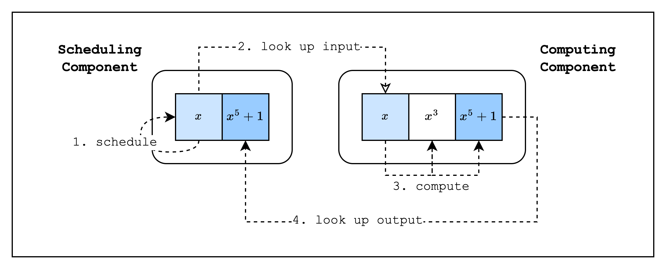
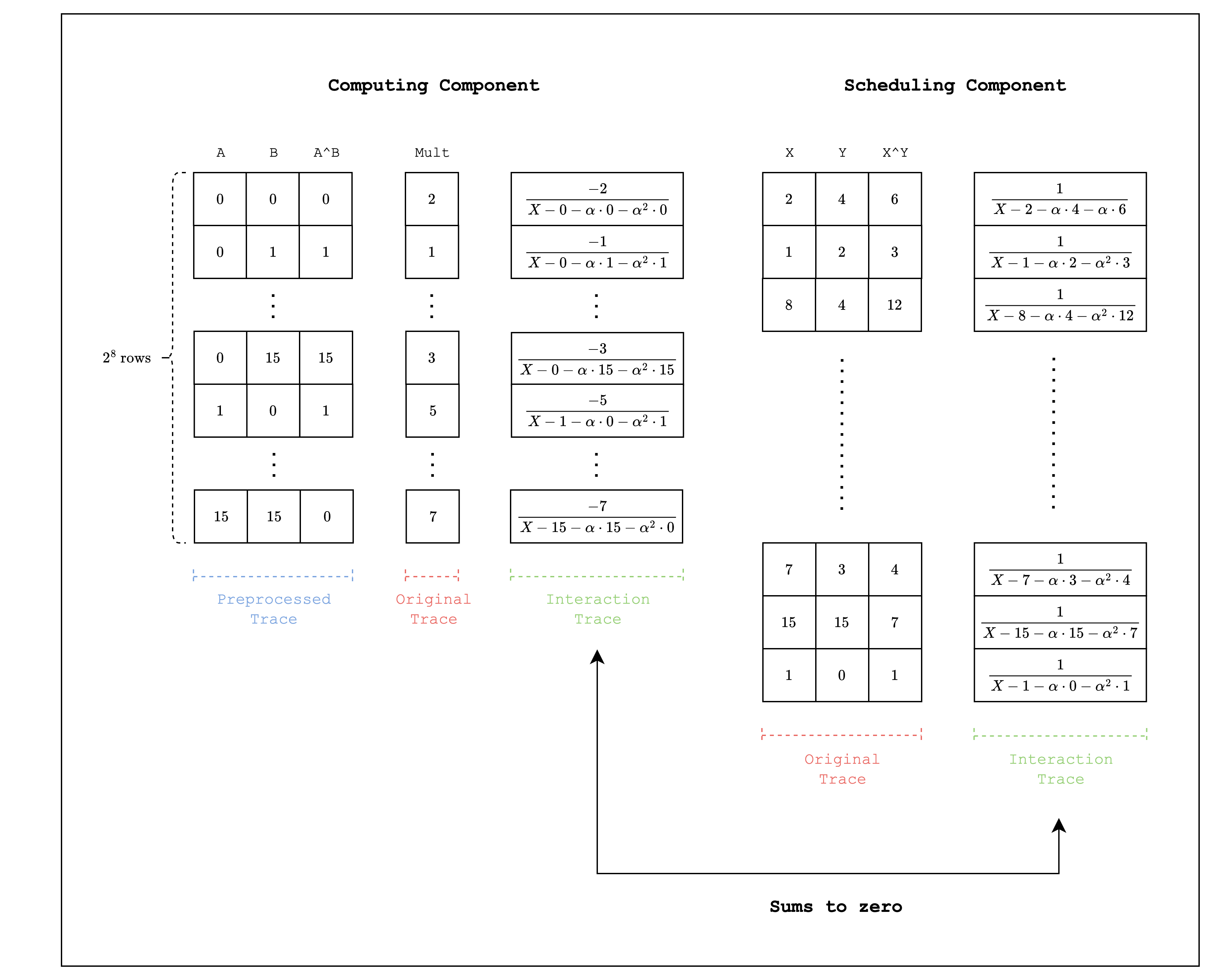
To illustrate how to use components, we will create two components where the main component calls a hash function component. For simplicity, instead of an actual hash function, the second component will compute from an input . This component will have, in total, three columns: [input, intermediate, output], which will correspond to the values . Our main component, on the other hand, will have two columns, [input, output], which corresponds to the values .
We'll refer to the main component as the scheduling component and the hash function component as the computing component, since the main component is essentially scheduling the hash function component to run its function with a given input and the hash function component computes on the provided input. As can be seen in Figure 1, the input and output of each component are connected by lookups.
Design
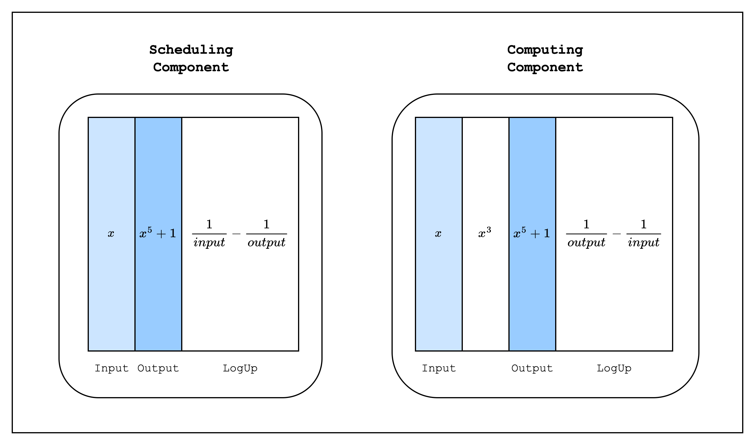
When we implement this in Stwo, the traces of each component will look like Figure 2 above. Each component has its own original and LogUp traces, and the inputs and outputs of each component are connected by lookups. Since the scheduling component sets the LogUp value as a positive multiplicity and the computing component sets the same value as a negative multiplicity, the verifier can simply check that the sum of the two LogUp columns is zero. Note that we combine the input and output randomly as
to form a single lookup. This is because we want to ensure that each input is paired with the correct output. If we add the input and output as separate lookups as
A malicious prover can switch the output with a different row and still come up with a valid proof. For example, the following scheduling component
| Input | Output |
|---|---|
| x | y^5 + 1 |
| y | x^5 + 1 |
And the following computing component
| Input | Intermediate | Output |
|---|---|---|
| x | x^3 + 1 | x^5 + 1 |
| y | y^3 + 1 | y^5 + 1 |
would be valid.
Implementation
Let's move on to the implementation.
fn main() {
    // --snip--

    // Create trace columns
    let scheduling_trace = gen_scheduling_trace(log_size);
    let computing_trace = gen_computing_trace(log_size, &scheduling_trace[0], &scheduling_trace[1]);

    // Statement 0
    let statement0 = ComponentsStatement0 { log_size };
    statement0.mix_into(channel);

    // Commit to the trace columns
    let mut tree_builder = commitment_scheme.tree_builder();
    tree_builder.extend_evals([scheduling_trace.clone(), computing_trace.clone()].concat());
    tree_builder.commit(channel);

    // Draw random elements to use when creating the random linear combination of lookup values in the LogUp columns
    let lookup_elements = ComputationLookupElements::draw(channel);

    // Create LogUp columns
    let (scheduling_logup_cols, scheduling_claimed_sum) = gen_scheduling_logup_trace(
        log_size,
        &scheduling_trace[0],
        &scheduling_trace[1],
        &lookup_elements,
    );
    let (computing_logup_cols, computing_claimed_sum) = gen_computing_logup_trace(
        log_size,
        &computing_trace[0],
        &computing_trace[2],
        &lookup_elements,
    );

    // Statement 1
    let statement1 = ComponentsStatement1 {
        scheduling_claimed_sum,
        computing_claimed_sum,
    };
    statement1.mix_into(channel);

    // Commit to the LogUp columns
    let mut tree_builder = commitment_scheme.tree_builder();
    tree_builder.extend_evals([scheduling_logup_cols, computing_logup_cols].concat());
    tree_builder.commit(channel);

    let components = Components::new(&statement0, &lookup_elements, &statement1);

    let stark_proof = prove(&components.component_provers(), channel, commitment_scheme).unwrap();

    let proof = ComponentsProof {
        statement0,
        statement1,
        stark_proof,
    };

    // --snip--
}
The code above for proving the components should look pretty familiar by now. Since we need to do everything twice as many times, we create structs like ComponentsStatement0, ComponentsStatement1, Components, and ComponentsProof, but the main logic is the same.
Let's take a closer look at how the LogUp columns are generated.
fn gen_scheduling_logup_trace(
    log_size: u32,
    scheduling_col_1: &CircleEvaluation<SimdBackend, M31, BitReversedOrder>,
    scheduling_col_2: &CircleEvaluation<SimdBackend, M31, BitReversedOrder>,
    lookup_elements: &ComputationLookupElements,
) -> (
    Vec<CircleEvaluation<SimdBackend, M31, BitReversedOrder>>,
    SecureField,
) {
        // --snip--

        let scheduling_input_output: PackedSecureField =
            lookup_elements.combine(&[scheduling_col_1.data[row], scheduling_col_2.data[row]]);
        col_gen.write_frac(row, PackedSecureField::one(), scheduling_input_output);

        // --snip--


fn gen_computing_logup_trace(
    log_size: u32,
    computing_col_1: &CircleEvaluation<SimdBackend, M31, BitReversedOrder>,
    computing_col_3: &CircleEvaluation<SimdBackend, M31, BitReversedOrder>,
    lookup_elements: &ComputationLookupElements,
) -> (
    Vec<CircleEvaluation<SimdBackend, M31, BitReversedOrder>>,
    SecureField,
) {
        // --snip--

        let computing_input_output: PackedSecureField =
            lookup_elements.combine(&[computing_col_1.data[row], computing_col_3.data[row]]);
        col_gen.write_frac(row, -PackedSecureField::one(), computing_input_output);

        // --snip--
}
As you can see, the LogUp values of the input and output columns of both the scheduling and computing components are batched together, but in the scheduling component, the output LogUp value is subtracted from the input LogUp value, while in the computing component, the input LogUp value is subtracted from the output LogUp value. This means that when the LogUp sums from both components are added together, they should cancel out to zero.
Next, let's check how the constraints are created.
impl FrameworkEval for SchedulingEval {
    // --snip--

    fn evaluate<E: EvalAtRow>(&self, mut eval: E) -> E {
        let input_col = eval.next_trace_mask();
        let output_col = eval.next_trace_mask();

        eval.add_to_relation(RelationEntry::new(
            &self.lookup_elements,
            E::EF::one(),
            &[input_col, output_col],
        ));

        eval.finalize_logup();

        eval
    }
}

impl FrameworkEval for ComputingEval {
    // --snip--

    fn evaluate<E: EvalAtRow>(&self, mut eval: E) -> E {
        let input_col = eval.next_trace_mask();
        let intermediate_col = eval.next_trace_mask();
        let output_col = eval.next_trace_mask();

        eval.add_constraint(
            intermediate_col.clone() - input_col.clone() * input_col.clone() * input_col.clone(),
        );
        eval.add_constraint(
            output_col.clone()
                - intermediate_col.clone() * input_col.clone() * input_col.clone()
                - E::F::one(),
        );

        eval.add_to_relation(RelationEntry::new(
            &self.lookup_elements,
            -E::EF::one(),
            &[input_col, output_col],
        ));

        eval.finalize_logup();

        eval
    }
}
As you can see, we define the LogUp constraints for each component, and we also add two constraints that make sure the computations and are correct.
fn main() {
    // --snip--

    // Verify claimed sums
    assert_eq!(
        scheduling_claimed_sum + computing_claimed_sum,
        SecureField::zero()
    );

    // Unpack proof
    let statement0 = proof.statement0;
    let statement1 = proof.statement1;
    let stark_proof = proof.stark_proof;

    // Create channel and commitment scheme
    let channel = &mut Blake2sChannel::default();
    let commitment_scheme = &mut CommitmentSchemeVerifier::<Blake2sMerkleChannel>::new(config);
    let log_sizes = statement0.log_sizes();

    // Preprocessed columns.
    commitment_scheme.commit(stark_proof.commitments[0], &log_sizes[0], channel);

    // Commit to statement 0
    statement0.mix_into(channel);

    // Trace columns.
    commitment_scheme.commit(stark_proof.commitments[1], &log_sizes[1], channel);

    // Draw lookup element.
    let lookup_elements = ComputationLookupElements::draw(channel);

    // Commit to statement 1
    statement1.mix_into(channel);

    // Interaction columns.
    commitment_scheme.commit(stark_proof.commitments[2], &log_sizes[2], channel);

    // Create components
    let components = Components::new(&statement0, &lookup_elements, &statement1);

    verify(
        &components.components(),
        channel,
        commitment_scheme,
        stark_proof,
    )
    .unwrap();
Finally, we verify the components!
Additional Examples
Here, we introduce some additional AIRs that may help in designing more complex AIRs.
Selectors
A selector is a column of 0s and 1s that selectively enables or disables a constraint. One example of a selector is the IsFirst column which has a value of 1 only on the first row. This can be used when constraints are defined over both the current and previous rows but we need to make an exception for the first row.
For example, as seen in Figure 1, when we want to track the cumulative sum of a column, i.e. , the previous row of the first row points to the last row, creating an incorrect constraint . Thus, we need to disable the constraint for the first row and enable a separate constraint . This can be achieved by using a selector column that has a value of 1 on the first row and 0 on the other rows and multiplying the constraint by the selector column:
where refers to the previous value of in the multiplicative subgroup of the finite field.
IsZero
Checking that a certain field element is zero is a common use case when writing AIRs. To do this efficiently, we can use the property of finite fields that a non-zero field element always has a multiplicative inverse.
For example, in Figure 2, we want to check whether a field element in is zero. We create a new column that contains the multiplicative inverse of each field element . We then use the multiplication of the two columns and check whether the result is 0 or 1. Note that if the existing column has a zero element, we can insert any value in the new column since the multiplication will always be zero.
This way, we can create a constraint that uses the IsZero condition as part of the constraint, e.g. , which checks if is 0 and if is not 0.
Public Inputs
When writing AIRs, we may want to expose some values in the trace to the verifier to check in the open. For example, when running an AIR for a Cairo program, we may want to check that the program that was executed is the correct one.
In Stwo, we can achieve this by adding the public input portion of the trace as a LogUp column as negative multiplicity. As shown in Figure 3, the public inputs are added as LogUp values with negative multiplicity and . The public inputs are given to the verifier as part of the proof and the verifier can directly compute the LogUp values with positive multiplicity and and add it to the LogUp sum and check that the total sum is 0.
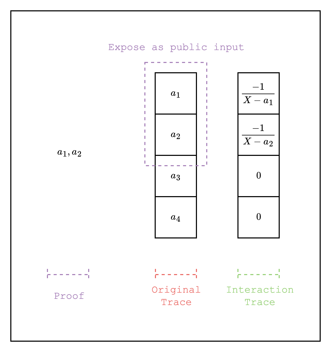
One important thing to note is that the public inputs must be added to the Fiat-Shamir channel before drawing random elements for the interaction trace. We refer the reader to this example implementation for reference.
XOR
We can also handle XOR operations as part of the AIR. First, as we did in the Components section, we create a computing component and a scheduling component. Then, we connect the two components using lookups: the computing component sets the LogUp value as a negative multiplicity and the scheduling component sets the same value as a positive multiplicity.
For example, Figure 4 shows the XOR operation for 4-bit integers. To accommodate the entire combination of inputs, the size of the trace for the computing component is rows. Note that the size of the trace for the scheduling component does not have to be the same as the computing component.
Note that for larger integers, we may need to decompose into smaller limbs to avoid creating large tables. Also note that the M31 field does not fully support XOR operations for 31-bit integers since we cannot use , although this is not feasible as it would require a table of size of around .
Cairo AIR
The following sections cover how Cairo is expressed as an AIR and proved using Stwo. The explanation is based on this commit of the Stwo-Cairo repository.
Overview of Cairo
This is an informal overview of Cairo. For a more formal explanation, please refer to the original Cairo paper.
Let's start by understanding how Cairo works. Essentially, Cairo is a Turing-complete CPU architecture specifically designed to enable efficient proofs of execution using STARKs. In particular, Cairo uses a read-only memory model instead of the more common read-write memory model and does not use any general-purpose registers.
Non-Deterministic Read-Only Memory
A read-only memory model is one where each address in memory can have only a single value throughout the program's execution. This contrasts with the more common read-write memory model, where an address can have multiple values at different points during execution.
The memory is also non-deterministic: the prover provides the values of the memory cells as witness values, and they do not need further constraints beyond ensuring that each address has a single value throughout the program's execution.
Registers
In physical CPUs, accessing memory is expensive compared to accessing registers due to physical proximity. This is why instructions typically operate over registers rather than directly over memory cells. In Cairo, accessing memory and registers incur the same cost, so Cairo instructions operate directly over memory cells. Thus, the three registers used by Cairo do not store instructions or operand values like in physical CPUs, but rather pointers to the memory cells where the instructions and operands are stored:
pcis the program counter, which points to the current Cairo instructionapis the allocation pointer, which points to the current available memory addressfpis the frame pointer, which points to the current frame in the "call stack"
Cairo Instructions
Let's now see what a Cairo instruction looks like.
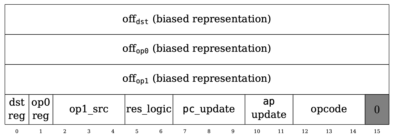
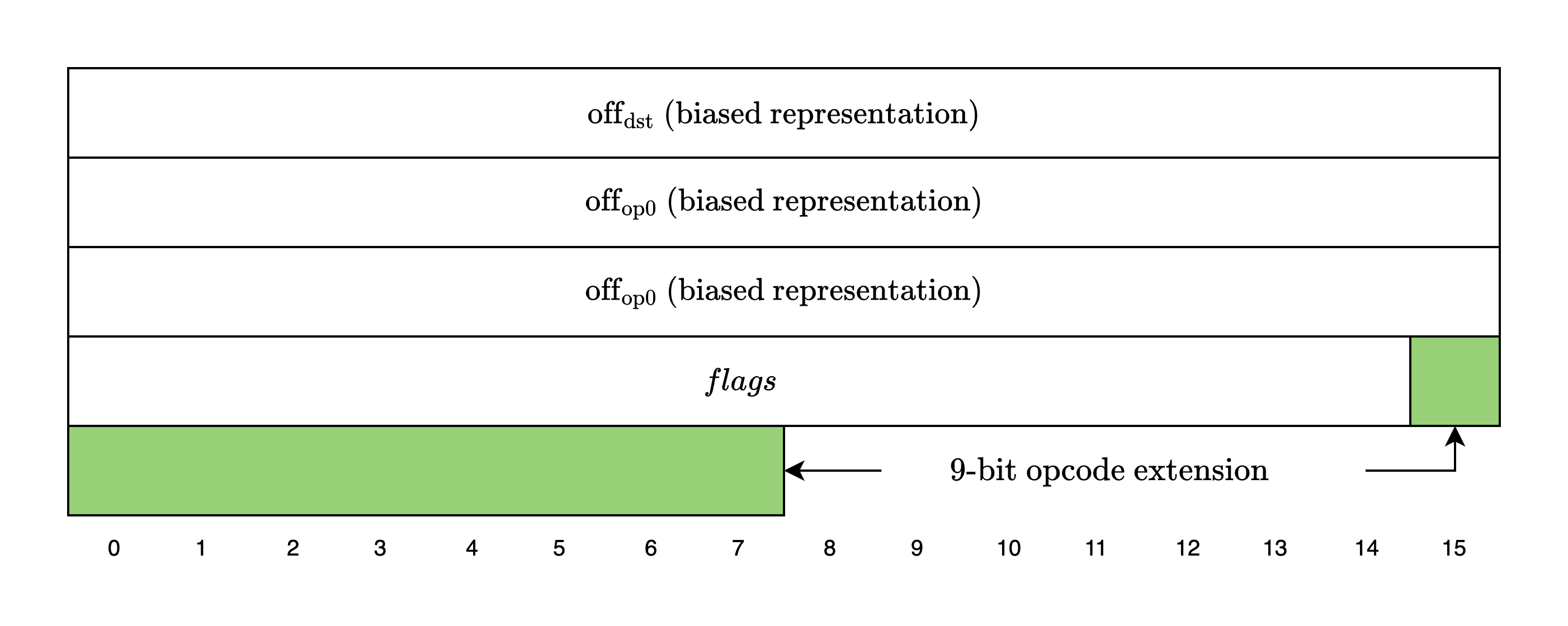
As the figure above from the Cairo paper shows, an instruction is 64 bits, where the first three 16-bit integers are signed offsets to the operands dst, op0, and op1.
The next 15 bits are flags. The dst_reg and op0_reg 1-bit flags indicate whether to use the ap or the fp register as the base for the dst and op0 operands. The op1_src flag supports a wider range of base values for the op1 operand: op0, pc, fp, and ap. The res_logic flag indicates how to compute the res operand: op1, op0 + op1, or op0 * op1. The pc_update and ap_update flags show how to update the pc and ap registers after computing the operands. The opcode flag indicates whether this instruction belongs to a predefined opcode (e.g., CALL, RET, ASSERT_EQ) and also defines how the ap and fp registers should be updated.
For a more detailed explanation of the flags, please refer to Section 4.5 of the Cairo paper.
Finally, the last bit is fixed to 0, but as we will see in the next section, this design has been modified in the current version of Cairo to support opcode extensions.
Opcodes and Opcode Extensions
In Cairo, an opcode refers to what the instruction should do. Cairo defines a set of common CPU operations as specific opcodes (e.g., ADD, MUL, JUMP, CALL), and the current version of Cairo also defines a new set of opcodes used to improve the performance of heavy computations such as Blake2s hashing and QM31 addition and multiplication.
Since the 64-bit instruction structure is not flexible enough to support this extended set of opcodes, Cairo extends the instruction size to 72 bits and uses the last 9 bits as the opcode extension value.
As of this commit, the following opcode extension values are supported:
0: Stone (original opcodes)1: Blake2: BlakeFinalize3: QM31Operation
Even if an instruction does not belong to any predefined set of opcodes, it is considered a valid opcode as long as it adheres to the state-transition function defined in Section 4.5 of the Cairo paper. In Stwo Cairo, this is referred to as a generic opcode.
Basic Building Blocks
This section covers the basic building blocks used to build the Cairo AIR.
Felt252 to M31
Cairo works over the prime field , while Stwo works over the prime field . Thus, in order to represent the execution of Cairo with Stwo, we need to decompose the 252-bit integers into 31-bit integers. The Cairo AIR chooses to use the 9-bit decomposition, so a single 252-bit integer will result in 28 9-bit limbs.
Range checks
Range-checks are very commonly used in the Cairo AIR. They are used to ensure that the witness values are within a certain range, most commonly within a certain bit length. For example, in the Felt252 to M31 section, we saw that a 252-bit integer is decomposed into 28 9-bit limbs, so we need to verify that each limb is in the range .
This is done by using a preprocessed column that contains the entire range of possible values for the bit length. For example, for a 9-bit range check, the column will contain the values from 0 to . We also have another column that contains the number of times the range-check was invoked for each valid value and we use lookups to check that each range-check is valid. For a more practical example, please refer to the Static Lookups section.
Main Components
Now that we have a basic understanding of Cairo and the building blocks that are used to build the Cairo AIR, let's take a look at the main components of the Cairo AIR.
For readers who are unfamiliar with the concepts of components and lookups, we suggest going over the Components section of the book.
Fetch, Decode, Execute
Cairo follows the common CPU architecture of fetching, decoding, and executing an instruction in a single CPU step. Below is a high-level diagram of what a single CPU step looks like in Cairo.
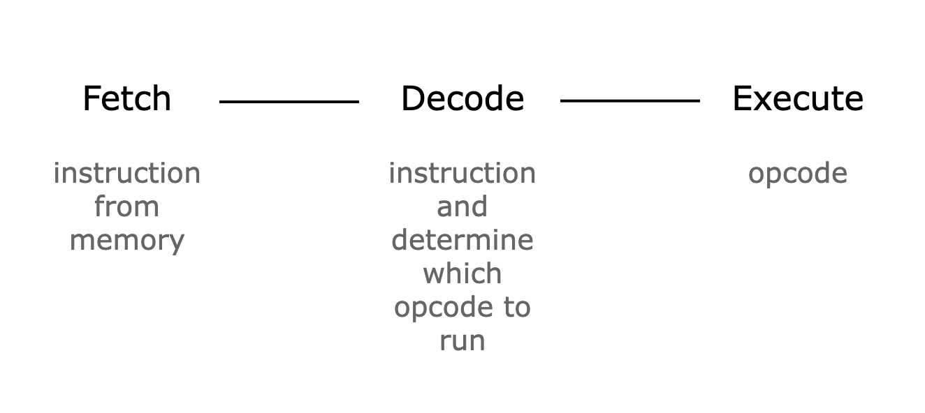
Since we need to prove the correctness of all CPU steps, the Cairo AIR writes the results of fetching, decoding, and executing an instruction at every CPU step into a trace and proves that the constraints over the trace are satisfied—i.e., consistent with the semantics of Cairo.
Let's keep this in mind while we go over the main components of the Cairo AIR.
1. Memory Component
The first component we need is a Memory component, which implements the non-deterministic read-only memory model of Cairo.
In Cairo AIR, instead of mapping the memory address to a value directly, we first map the address to an id and then map the id to a value. This is done to classify the memory values into two groups: Small and Big, where Small values are 72-bit integers and Big values are 252-bit integers. As many memory values do not exceed the Small size, this allows us to save cost on unnecessary padding.
As a result, the Memory component is actually 2 components: MemoryAddressToId and MemoryIdToValue.
The constraints for the MemoryAddressToId and MemoryIdToValue components are as follows:
- An
addressmust appear once and only once in theMemoryAddressToIdcomponent. - An
idmust appear once and only once in theMemoryIdToValuecomponent. - Each
(address, id, value)tuple must be unique.
The first constraint is implemented by using a preprocessed column that contains the sequence of numbers [0, MAX_ADDRESS) and using this as the address values (in the actual code, the memory address starts at 1, so we need to add 1 to the sequence column).
The second constraint is guaranteed because the address value is always unique.
A short explainer on how the id value is computed:
The id value is a 31-bit integer that is incremented by 1 from 0 whenever there is a unique memory access. For example, if the addresses [5, 1523, 142] were accessed in that order, the ids for those addresses will be (5, 0), (1523, 1), and (142, 2).
Since an id value needs to include information as to whether the corresponding value is Small or Big, we use the MSB as a flag (0 for Small and 1 for Big). Thus, an id value that corresponds to a Small value can occupy the space [0, 2^30), while an id value that corresponds to a Big value can occupy the space [2^30, 2^31).
In reality, the size of each table will be [0, NUM_SMALL_VALUES_ACCESSED) and [2^30, 2^30 + NUM_BIG_VALUES_ACCESSED), where NUM_SMALL_VALUES_ACCESSED and NUM_BIG_VALUES_ACCESSED are values that are provided by the prover. To make sure that the id values are created correctly, we can use the preprocessed column as the id values.
2. VerifyInstruction Component
The VerifyInstruction component is responsible for accessing the instruction from the Memory component and decomposing the retrieved value. As mentioned in the Felt252 to M31 section, a 252-bit integer is stored as 28 9-bit limbs, so we need to decompose the limbs and concatenate them to get the values we need. For example, as in Figure 2 in order to get the 3 16-bit offset values, we need to decompose the first 6 limbs into [9, [7, 2], [9], [5, 4], [9], [3, 6]] and concatenate them as the following: [[9, 7], [2, 9, 5], [4, 9, 3]]. Then, the remaining 6-bit value and the next limb will correspond to the 15-bit flags, and the next (8th) limb will be the opcode extension value. The other 20 limbs should all be zeros. At the end, we will have decomposed the instruction value into 3 16-bit offsets, 2 chunks of flags, and a 9-bit opcode extension.
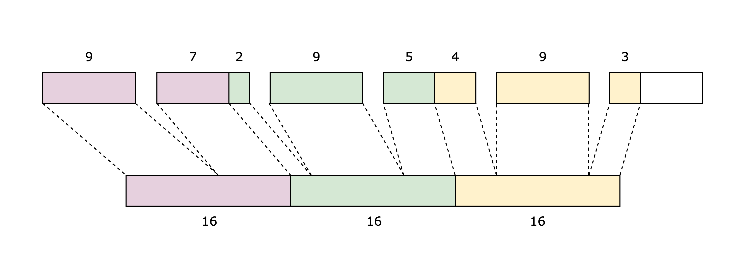
Note that the decomposition will be constrained by range checking that each integer is within its corresponding range.
3. Opcode Component
Since every Cairo instruction can be mapped to a specific Opcode, we can check that a Cairo instruction is executed by checking that the corresponding Opcode component was executed correctly. You can think of the Opcode component as the main component that uses the VerifyInstruction and Memory components.
We define a single Opcode component for each predefined opcode and a GenericOpcode component, which is used for all instructions that do not map to any of the predefined opcodes.
The following is a list of constraints that the Opcode component needs to verify:
- The offsets and flag values are correct using the
VerifyInstructioncomponent. - The instruction is correctly mapped to the current
Opcodecomponent using the flags. - The operand values
op0,op1, anddstcomputed with the registers and the offsets are correct using theMemorycomponent. - The operation for the current
Opcodecomponent is done correctly. - The state transition of the three registers (
pc,ap,fp) is done correctly using the flags.
Of these constraints, items 2 and 4 are self-contained—meaning they do not require any other components to be verified. We will explore how the remaining three are verified using lookups between the different components.
Bringing It All Together
The following figure shows how each of the main components are connected to each other using lookups.
If we look at the right-hand side first, we can see the main components of the Cairo AIR. The boxes in each component correspond to lookups within that component, and boxes with the same fill color correspond to lookups of the same values. Some lookups are yielded (i.e., subtracted), while others are used (i.e., added). Yielded lookups have red edges; used lookups have blue edges.
On the left-hand side, we can see lookups that are computed directly by the verifier from data provided by the prover as part of the proof.
Each component has a claimed sum value that corresponds to the sum of all the lookups in the component. These claimed sums are provided by the prover as part of the proof, and the verifier adds them together along with the lookups on the left-hand side. If the total sum is zero, the verifier is convinced that the proof is valid.
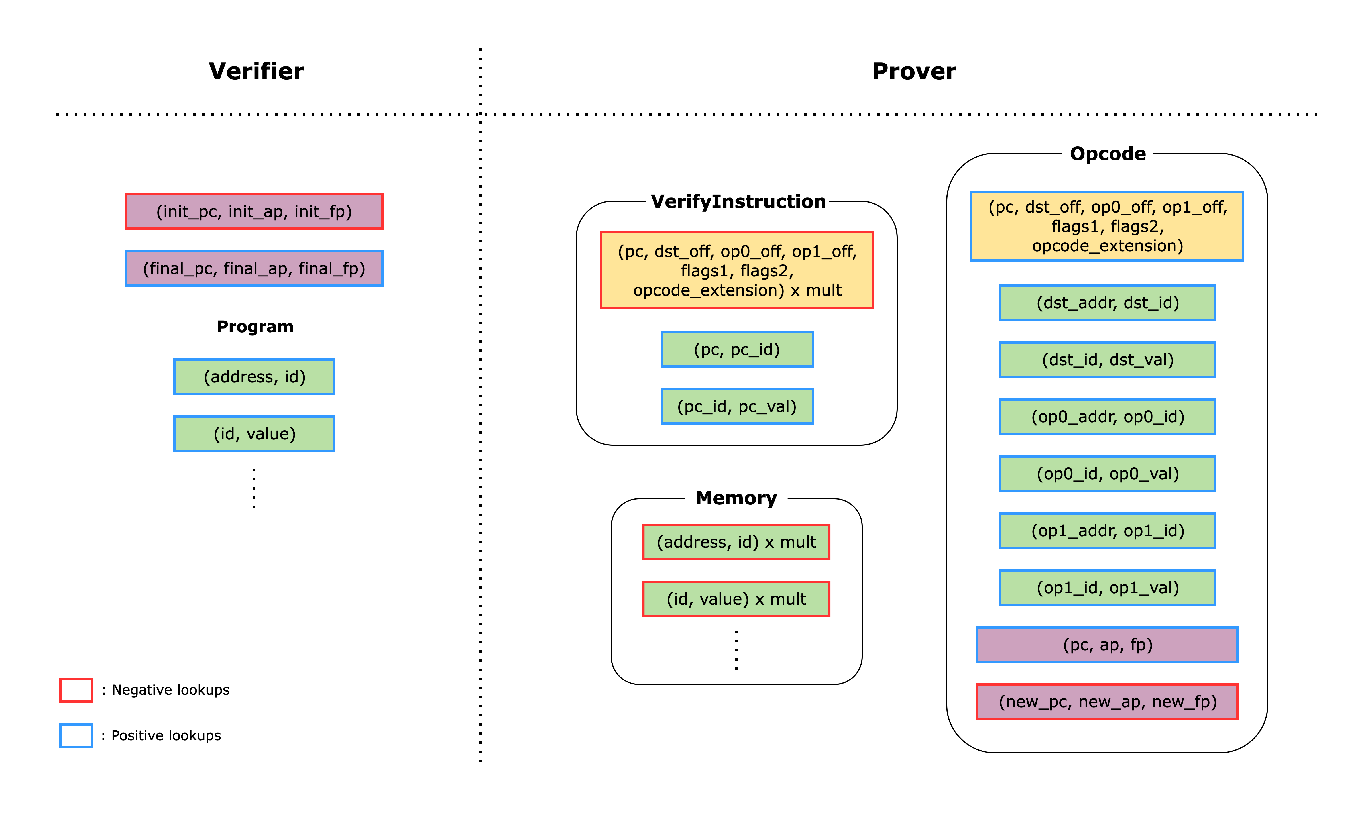
Memory Lookups
The memory lookups correspond to looking up the (address, id) and (id, value) pairs. In the Memory component, each of the lookups is multiplied by a witness value mult, which indicates the number of times each memory address was accessed. Since the memory accesses are added to the total sum and the same amount is subtracted from the total sum in the Memory component, the total sum for memory lookups should equal zero.
Note that the verifier also adds lookups for the Cairo program, which is necessary to ensure that the correct program is actually stored in memory and is properly executed.
Instruction Lookups
Once the VerifyInstruction component retrieves the instruction value using the (pc_addr, pc_id) and (pc_id, pc_val) lookups, it subtracts the lookup of the tuple (pc, dst_off, op0_off, op1_off, flags1, flags2, opcode_extension), which are the decomposed values of the instruction. This lookup also has a mult witness because the VerifyInstruction component has a single row for each unique pc value (i.e., the Cairo instruction stored at the pc address). Thus, the same pc value can be invoked multiple times throughout the program, and the mult value represents the number of times the same pc value is invoked.
Since the same tuple lookup is added to the total sum whenever the Opcode component uses the same instruction, the total sum for instruction lookups should equal zero.
Register Lookups
After computing over the operands, a Cairo instruction updates the register values based on the values in the flags. In an Opcode component, this update logic is verified using the columns pc, ap, fp, new_pc, new_ap, new_fp, and by constraining the values with the flags.
In addition to checking that each state transition is done correctly, we also need to make sure that the initial register values (i.e., before running the program) and the final register values (i.e., after running the program) satisfy the Cairo semantics. For example, the final pc must point to an instruction that runs the JUMPREL 0 opcode, which is an infinite loop (you can check the rest of the semantics enforced here).
Once we have verified that the initial and final register values are correct and each state transition is done correctly, we do a final check that the register values are all connected—that is, the register values used by the second instruction are the same as the new register values of the first instruction, and so on. We check this by adding the lookup of the (pc, ap, fp) tuple and subtracting the lookup of the (new_pc, new_ap, new_fp) tuple for each Opcode row. When we add up all the lookups, the total sum for register lookups should equal (init_pc, init_ap, init_fp) - (final_pc, final_ap, final_fp). Thus, the verifier can compute the lookups of the initial and final register values, subtract the first, add the second, and check that the total sum is zero.
ADD Opcode Walkthrough
To better understand how Opcode components work, let's walk through the implementation of the AddOpcode component.
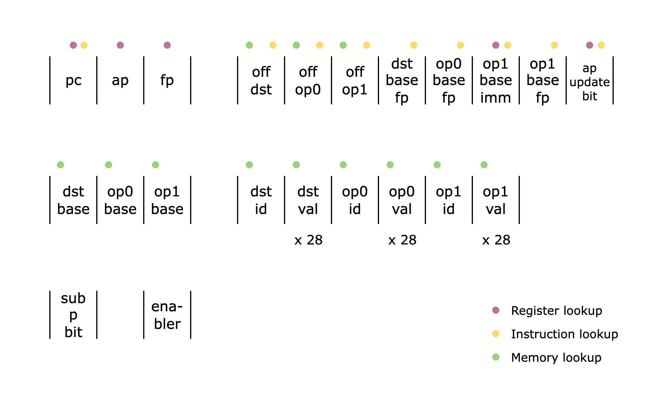
Above is the list of all the columns used in the AddOpcode component. Note that the dst_val, op0_val, and op1_val columns are actually 28 columns each (to support 28 9-bit limbs), but we show them as single columns for brevity.
To reiterate what an Opcode component does from the Main Components section, it verifies the following:
- The offsets and flag values are correct using the
VerifyInstructioncomponent. - The instruction is correctly mapped to the current
Opcodecomponent using the flags. - The operand values
op0,op1, anddstcomputed with the registers and the offsets are correct using theMemorycomponent. - The operation for the current
Opcodecomponent is done correctly. - The state transition of the three registers (
pc,ap,fp) is done correctly using the flags.
An instruction should contain 15 bits of flags but only 5 bits are represented in the AddOpcode columns. Can you see why?
Hint
Hint
Check out how a Cairo instruction is pattern-matched to an ADD opcode here.
Hint
Hint
Check out how the decomposition of the flags is verified here.
Items 1 and 3 should be familiar, as we already covered them in the Main Components section. For item 2, you can check the specs for the ADD opcode here. For item 5, the specs for a valid state transition can be found in Section 4.5 of the Cairo paper.
In this section, we will focus on how item 4 is implemented.
Adding two 252-bit integers
Assuming that the operands op0, op1, and dst are correctly accessed from the Memory table, we now check that the addition of two 252-bit integers is done correctly, i.e. op0 + op1 = dst. As noted in the Felt252 to M31 section, a 252-bit integer is stored as 28 9-bit limbs, so we need to check addition for each of the 28 limbs.
We will incrementally build up to the final constraint.
Limb-wise Addition and Carry
To verify that the two sets of limbs are correctly added, we check limb-wise addition. Since each limb can create a carry, we also add the carry from the previous limb (except for the first limb). Thus, the constraints look like this:
carry_limb_1 = (op0[0] + op1[0] - dst[0]) / 2^9
carry_limb_1 * (carry_limb_1 - 1) = 0

carry_limb_2 = (op0[1] + op1[1] + carry_limb_1 - dst[1]) / 2^9
carry_limb_2 * (carry_limb_2 - 1) = 0

...

op0[27] + op1[27] + carry_limb_27 - dst[27] = 0
We divide op0[0] + op1[0] - dst[0] by 2^9 since this quantity is either 2^9 (if a carry exists) or 0 (if no carry exists). Dividing by 2^9 yields one or zero, respectively. To check that the carry is either 0 or 1, we add the constraint carry_limb_0 * (carry_limb_0 - 1) = 0. For the final limb, we simply check that the addition is correct.
Handling overflow beyond the 252-bit prime field
We also need to account for addition overflowing the 252-bit prime field P (i.e., op0 + op1 = dst + P). To check this, we introduce a witness variable sub_p_bit, a 1-bit value set to 1 if there is an overflow. Note that since P = 2^251 + 17 * 2^192 + 1, we only subtract in the three limbs where P has a non-zero limb: 0, 22, 27.
Now let's revisit the constraints:
sub_p_bit * (sub_p_bit - 1) = 0

carry_limb_1 = (op0[0] + op1[0] - dst[0] - sub_p_bit) / 2^9
carry_limb_1 * (carry_limb_1 - 1) = 0

...

carry_limb_23 = (op0[22] + op1[22] + carry_limb_22 - dst[22] - sub_p_bit * 136) / 2^9
carry_limb_23 * (carry_limb_23 - 1) = 0

...

op0[27] + op1[27] + carry_limb_27 - dst[27] - sub_p_bit * 256 = 0
First, we verify that sub_p_bit is a bit. Then, we subtract sub_p_bit from the first limb, sub_p_bit * 136 from the 22nd limb, and sub_p_bit * 256 from the 27th limb. (Note that 136 and 256 are the values of P in the 22nd and 27th limbs, respectively.)
A caveat of this approach is that subtracting sub_p_bit can introduce an underflow, i.e., (op0[0] + op1[0] - dst[0] - sub_p_bit) / 2^9 = -1. This means that carry_limb_0 can be -1 as well as 0 or 1. Thus, we update the constraint for all carries to the following:
...

carry_limb_1 * (carry_limb_1 - 1) * (carry_limb_1 + 1) = 0

...
Optimization
To optimize the number of constraints, we can combine all the constraints for each limb into a single constraint. Naively checking that carry_limb_1 = (op0[0] + op1[0] - dst[0] - sub_p_bit) / 2^9 would require a dedicated column for carry_limb_1. Instead, we keep carry_limb_1 as an intermediate value and inline the equation when computing the next carry. For example, the second-limb carry is computed as follows:
carry_limb_2 = (op0[1] + op1[1] + ((op0[0] + op1[0] - dst[0] - sub_p_bit) / 2^9) - dst[1]) / 2^9
This way, we avoid allocating extra columns for the carries and proceed until the last limb, where we check that the giant equation is correct.
This is possible because the computation does not involve any multiplication of witness values, so the constraint degree does not blow up.
Final constraint
One last note: in the implementation, we replace division by 2^9 with multiplication by 2^22, which is equivalent in the M31 field since 2^9 and 2^22 are multiplicative inverses—i.e., 2^9 * 2^22 = 1 mod 2^31 - 1.
So the final constraint looks like this:
sub_p_bit * (sub_p_bit - 1) = 0

carry_limb_1 = (op0[0] + op1[0] - dst[0] - sub_p_bit) * 2^22 // intermediate representation
carry_limb_1 * (carry_limb_1 - 1) * (carry_limb_1 + 1) = 0

...

carry_limb_27 = (op0[26] + op1[26] + carry_limb_26 - dst[26]) * 2^22 // intermediate representation
carry_limb_27 * (carry_limb_27 - 1) * (carry_limb_27 + 1) = 0

op0[27] + op1[27] + carry_limb_27 - dst[27] - sub_p_bit * 256 = 0
Enabler column
Finally, we introduce the last column in the AddOpcode component: the enabler column. As the name suggests, this column enables or disables the constraint for the current row. It is used to support the dummy rows added to the end of the table to make the number of rows a power of two. In other words, it is set to 1 for all valid ADD opcode calls and 0 for all dummy rows.
Stwo: Under the Hood
This section provides an overview of the core components and protocols that make up Stwo. It is intended for readers who want to understand the technical details and inner workings of the system implementation. Throughout this section, we describe the implementation as available in this commit.
The following topics are covered:
- Mersenne Primes: Introduction to the Mersenne31 prime field used in Stwo for efficient arithmetic.
- Circle Group: Explains the algebraic structure underlying FFT and polynomial operations.
- Circle Polynomials: Details the representation and evaluation of polynomials in the circle group.
- Circle FFT: Describes the fast Fourier transform algorithm adapted for the circle group.
- Vector Commitment Scheme (VCS): Covers the use of Merkle trees for committing to vectors and enabling efficient proofs of inclusion.
- AIR to Composition Polynomial: Shows how algebraic constraints are encoded as polynomials for proof generation.
- Circle FRI: Explains the FRI protocol for low-degree testing of polynomials over the circle group.
- Polynomial Commitment Scheme (PCS): Describes the protocol for committing to and opening polynomials with soundness guarantees.
- Proof Generation and Verification: Walks through the process of generating and verifying a STARK proof in Stwo.
- Lookups: Discusses lookup arguments and their implementation in Stwo for efficient constraint checking.
Mersenne Primes
Proof systems typically rely on finite field operations, where efficient field arithmetic is crucial for optimizing proof generation. In STARK protocols, there is no direct dependency between the security level of the proof system and the field size. This allows the use of small fields with highly efficient arithmetic.
Stwo uses a particular family of primes called Mersenne primes. A Mersenne prime is defined as a prime number that is one less than a power of two, expressed as . Stwo uses the Mersenne prime of size , which is implemented as follows:
pub struct M31(pub u32);Why ?
The key advantage is extremely cheap modular reduction after a 31-bit multiplication. Consider computing , where . This operation involves a 31-bit integer multiplication, producing a 62-bit intermediate result, which is then reduced modulo .
Suppose then we can decompose into two 31-bit values and , such that , as shown in the following figure.

To perform modular reduction, we start with: Substituting gives:
Since and are both 31-bit values, they can be directly represented as field elements. Consequently, modular reduction is performed with a single field addition. This makes arithmetic over Mersenne primes exceptionally fast, making them an ideal choice for our STARK protocol. The above field multiplication is implemented as:
    fn mul(self, rhs: Self) -> Self::Output {
        Self::reduce((self.0 as u64) * (rhs.0 as u64))
    }
where reduce is a function which performs efficient reduction of the resulting number modulo .
Why We Need Extensions ?
We cannot instantiate our STARK protocols using since it is not FFT-friendly field, meaning it does not contain a multiplicative subgroup of order that is a large power of two (commonly referred to as a smooth subgroup). The multiplicative group of has the following order:
As shown above, the multiplicative group of lacks a smooth subgroup of size that is a large power of two because there is no large power of two that divides . In other words, there does not exist a sufficiently large such that . To make compatible with STARKs, we will work over extensions of it.
Field Operations
Stwo avoids code duplication by providing two Rust macros, impl_field! and impl_extension_field!, for implementing field and extension field operations.
For example, field operations for are implemented using the Rust macro impl_field!, which takes as argument the field and the size of the field , as follows:
impl_field!(M31, P);Since we work over extensions of , it has the type alias BaseField, as follows:
pub type BaseField = M31;Extensions of Mersenne Prime Field
This section describes two extensions of : complex extension and quartic extension.
Complex Extension
We construct the degree-2 extension of denoted by using the polynomial which is irreducible over .
This extension forms a field of size , where elements can be represented as or where and is the root of the polynomial i.e. . This is implemented as follows:
pub struct CM31(pub M31, pub M31);The order of the multiplicative group of is calculated as follows:
As shown above, i.e. the multiplicative group of contains a subgroup of size that is a large power of two. This makes it suitable for instantiating STARKs. This subgroup is what we refer to as the Circle group (explored further in the next section).
Similar to , the operations of are defined using the macros impl_field! and impl_extension_field! (which takes as argument the field and the field to be extended i.e. ). These are implemented as follows:
impl_field!(CM31, P2);
impl_extension_field!(CM31, M31);
where P2 is the size of i.e. .
Quartic Extension
For the soundness of the protocol, it is crucial that the verifier samples random challenges from a sufficiently large field to ensure that an adversary cannot guess or brute-force the challenges and generate a proof that passes verification without knowledge of the witness.
If we use , then 31-bit random challenges are not sufficient to maintain the security of the protocol. To address this, the verifier draws random challenges from a degree-4 extension of denoted by , which is equivalent to degree-2 extension of , denoted as
Here the polynomial is irreducible over .
The elements of can be represented as or where and is the root of the polynomial i.e. . This is implemented as follows:
pub struct QM31(pub CM31, pub CM31);
pub type SecureField = QM31;
Since the verifier uses the field to sample random challenges it is given the type alias SecureField.
Alternatively, the elements of can also be represented as four elements of i.e. or
where . With four elements from , the challenge space consists of 124-bit values, offering a sufficiently large possibilities to sample a random challenge.
Similar to , the operations of are defined using the macros impl_field! and impl_extension_field!, implemented as follows:
impl_field!(QM31, P4);
impl_extension_field!(QM31, CM31);
where P4 is the size of i.e. .
In the next section, we will explore the circle group, which is used to instantiate the STARK protocol.
Circle Group
As discussed in the previous section, Mersenne prime field lacks a smooth subgroup whose order is a large power of two. This property makes such fields unsuitable for instantiating STARK protocols. To address this, we consider extensions of that have smooth subgroups, which are suitable for performing FFTs and implementing the FRI protocol.
For a field extension of , we define the circle curve as the set of points satisfying the relation:
In Stwo implementation, a point on the circle is defined as follows:
pub struct CirclePoint<F> {
    pub x: F,
    pub y: F,
}
The set forms a cyclic group under the operation defined by:
Here, the group is defined additively, which differs from the multiplicative notation used in the Circle STARKs paper. In this documentation, we adopt the additive notation for consistency with the implementation. The above group operation is implemented as:
    fn add(self, rhs: Self) -> Self::Output {
        let x = self.x.clone() * rhs.x.clone() - self.y.clone() * rhs.y.clone();
        let y = self.x * rhs.y + self.y * rhs.x;
        Self { x, y }
    }
The identity element in this group is , implemented as:
    pub fn zero() -> Self {
        Self {
            x: F::one(),
            y: F::zero(),
        }
    }
Negation in the circle group corresponds to the conjugation map , defined by:
This is same as complex conjugation in complex numbers. In Stwo, the conjugate of a CirclePoint is computed as:
    pub fn conjugate(&self) -> CirclePoint<F> {
        Self {
            x: self.x.clone(),
            y: -self.y.clone(),
        }
    }
The total number of points in the circle group is given by . Specifically, for , the number of points is , which, as discussed earlier, is a large power of two and can thus be used in STARK protocol instantiations. This result is proven in Lemma 1 of the Circle STARKs paper.
In Stwo implementation, the generator of the group is defined as: Subgroups of of size can be generated using the following function:
    pub fn subgroup_gen(n: u32) -> CirclePoint<F> {
        assert!(n <= M31_CIRCLE_LOG_ORDER); // M31_CIRCLE_LOG_ORDER = 31
        let s = 1 << (M31_CIRCLE_LOG_ORDER - n);
        M31_CIRCLE_GEN.mul(s) // M31_CIRCLE_GEN = g = (2, 1268011823)
    }
To generate a subgroup of size , the function computes , i.e. it applies the group law to the generator with itself times, as shown below:
    pub fn mul(&self, mut scalar: u128) -> CirclePoint<F> {
        let mut res = Self::zero();
        let mut cur = self.clone();
        while scalar > 0 {
            if scalar & 1 == 1 {
                res = res + cur.clone();
            }
            cur = cur.double();
            scalar >>= 1;
        }
        res
    }
Hence, the point serves as a generator of a subgroup of order .
Circle Domain
In a STARK protocol, the computation trace is interpolated as a low-degree polynomial over a domain using FFT. For Circle STARKs, this domain consists of points on the circle curve and is referred to as the circle domain. The circle domain of size is constructed as the union of two disjoint cosets: Here, is a subgroup of size , and is the coset offset such that . This union is also called the twin-coset. The second coset in the union can be viewed as the negation (or conjugation) of the first: Therefore, it suffices to store only the half coset , and generate the full domain via its conjugates. The circle domain is defined in Stwo as:
pub struct CircleDomain {
    pub half_coset: Coset,
}
The following figure shows a circle domain of size 8. It is constructed from the half coset of size 4 (shown as red points) and its negation (shown as blue points).

To iterate over all points in the circle domain, we can iterate over the half coset and its conjugates:
    pub fn iter(&self) -> CircleDomainIterator {
        self.half_coset
            .iter()
            .chain(self.half_coset.conjugate().iter())
    }
Canonic Coset
For a specific choice of offset , the twin-coset becomes a coset of a larger subgroup. In particular, if is a generator of a subgroup of order , then: This result is proven in Proposition 1 of the Circle STARKs paper. Such domains are called standard position coset, or are referred to as canonic cosets. They are implemented as follows:
pub struct CanonicCoset {
    pub coset: Coset,
}
Here, CanonicCoset represents the full coset , while CircleDomain is represented with its half coset . Thus to compute the CircleDomain from the CanonicCoset, first calculate the half coset , which will be used to initialize the CircleDomain as shown below:
    pub fn circle_domain(&self) -> CircleDomain {
        CircleDomain::new(self.half_coset())
    }
The following figure shows a canonic coset of size 8. It is constructed from the coset of size 8 followed by an offset by , where is the generator of subgroup .

We can verify whether a given CircleDomain is canonic by checking the step size of the half coset against the initial coset offset. In the CircleDomain implementation, only the half coset is explicitly stored. If CircleDomain is canonic, must be a generator of the subgroup , which has order i.e. . Recall that the generator of the subgroup is .
Thus, the step size between consecutive elements in the half coset is , and the initial point is . Therefore, the ratio between the step size and the initial coset offset is:
This means that in a canonic coset, the step size is exactly four times the initial coset offset. This condition is used to check whether a CircleDomain is canonic, as shown below:
    pub fn is_canonic(&self) -> bool {
        self.half_coset.initial_index * 4 == self.half_coset.step_size
    }
In the next section, we will dive into polynomials defined over the circle.
Circle Polynomials
In STARK protocols, the computation trace is organized into columns and represented as polynomials. This section explains how Stwo represents and manipulates polynomials over the circle, covering both point-value (evaluations) and coefficient representations.
This section is organized as follows:
- Columns: How computation trace data is stored in columns, including both base field and secure field representations.
- Circle Evaluations and Polynomials: Point-value and coefficient representations of polynomials, their mathematical foundations, and conversion between forms.
- Secure Evaluations and Polynomials: Extension to secure field polynomials using the quartic extension QM31, with implementation details.
Columns
In Stwo, the computation trace is represented using multiple columns, each containing elements from the Mersenne prime field . The columns are defined via the Column<T> trait, where T is typically BaseField (an alias for M31).
pub trait Column<T>: Clone + Debug + FromIterator<T> {
    /// Creates a new column of zeros with the given length.
    fn zeros(len: usize) -> Self;
    /// Creates a new column of uninitialized values with the given length.
    /// # Safety
    /// The caller must ensure that the column is populated before being used.
    unsafe fn uninitialized(len: usize) -> Self;
    /// Returns a cpu vector of the column.
    fn to_cpu(&self) -> Vec<T>;
    /// Returns the length of the column.
    fn len(&self) -> usize;
    /// Returns true if the column is empty.
    fn is_empty(&self) -> bool {
        self.len() == 0
    }
    /// Retrieves the element at the given index.
    fn at(&self, index: usize) -> T;
    /// Sets the element at the given index.
    fn set(&mut self, index: usize, value: T);
}
The operations over a column such as bit reversal of elements is provided using the ColumnOps<T> trait, which also implements the type alias Col<B, T> to conveniently represent a column.
pub trait ColumnOps<T> {
    type Column: Column<T>;
    fn bit_reverse_column(column: &mut Self::Column);
}

pub type Col<B, T> = <B as ColumnOps<T>>::Column;Stwo defines a Backend trait, with two main implementations: CpuBackend and SimdBackend. The SimdBackend offers optimized routines for hardware supporting SIMD instructions, while CpuBackend provides a straightforward reference implementation.
Each backend implements the ColumnOps trait. Here and in the following sections, we will describe the trait implementations for the CpuBackend.
The ColumnOps<T> trait is implemented for the CpuBackend as follows:
impl<T: Debug + Clone + Default> ColumnOps<T> for CpuBackend {
    type Column = Vec<T>;

    fn bit_reverse_column(column: &mut Self::Column) {
        bit_reverse(column)
    }
}
Here, bit_reverse performs a naive bit-reversal permutation on the column.
Secure Field Columns
An element of the secure field (SecureField = QM31) cannot be stored in a single BaseField column because it is a quartic extension of M31. Instead, each secure field element is represented by four base field coordinates and stored in four consecutive columns.
pub struct SecureColumnByCoords<B: ColumnOps<BaseField>> {
    pub columns: [Col<B, BaseField>; SECURE_EXTENSION_DEGREE],
}
Here, SECURE_EXTENSION_DEGREE is the extension degree of QM31 i.e. 4. You can think of each row of the 4 columns containing a single element of the SecureField. Thus accessing an element by index reconstructs it from its base field coordinates, implemented as follows:
    pub fn at(&self, index: usize) -> SecureField {
        SecureField::from_m31_array(std::array::from_fn(|i| self.columns[i].at(index)))
    }
Now that we know how columns are represented, we can explore their use in storing evaluations over the circle domain and in interpolating polynomials.
Circle Evaluations and Polynomials
A polynomial can be represented in two main ways:
- Point-value representation: as evaluations over a domain
- Coefficient representation: as coefficients with respect to some basis
The conversion from point-value representation to coefficient representation is called interpolation and the conversion from coefficient representation to point-value representation is called evaluation. Both these conversions are based on fast Fourier transform (FFT), which will be covered in the upcoming sections.
In this subsection, we will look at the implementations of both these representations in Stwo and the respective functions defined on them to interpolate and evaluate polynomials.
Point-value representation
In Stwo, the evaluations of a polynomial over a CircleDomain are stored using the struct CircleEvaluation, implemented as follows:
pub struct CircleEvaluation<B: ColumnOps<F>, F: ExtensionOf<BaseField>, EvalOrder = NaturalOrder> {
    pub domain: CircleDomain,
    pub values: Col<B, F>,
    _eval_order: PhantomData<EvalOrder>,
}
Here, the domain (i.e. CircleDomain) and the evaluations (i.e. values) have the same ordering (i.e. EvalOrder) which can either be NaturalOrder or BitReversedOrder.
Now given the evaluations over a domain as CircleEvaluation we can interpolate a circle polynomial using the following functions:
impl<B: PolyOps> CircleEvaluation<B, BaseField, BitReversedOrder> {
    /// Computes a minimal [CirclePoly] that evaluates to the same values as this evaluation.
    pub fn interpolate(self) -> CirclePoly<B> {
        let coset = self.domain.half_coset;
        B::interpolate(self, &B::precompute_twiddles(coset))
    }

    /// Computes a minimal [CirclePoly] that evaluates to the same values as this evaluation, using
    /// precomputed twiddles.
    pub fn interpolate_with_twiddles(self, twiddles: &TwiddleTree<B>) -> CirclePoly<B> {
        B::interpolate(self, twiddles)
    }
}
Here, PolyOps is a trait that defines operations on BaseField polynomials, such as interpolation and evaluation. Now before looking into the representation of the circle polynomial (i.e. CirclePoly), let us first look into some theory on polynomials over the circle.
Polynomials over the circle
Let be an extension of the Mersenne prime field . Then represents the ring of bivariate polynomials with coefficients in . The circle polynomials are bivariate polynomials over quotient by the ideal . The space of these bivariate polynomials over the circle curve of total degree is denoted by .
For any polynomial , we can substitute all the higher degree terms of with the equation of circle and reduce to the form:
The above form is called the canonical representation of any polynomial . Since is of total degree , has degree and has degree . Thus an alternate representation of the space is as follows:
From the above representation we can see that the space is spanned by the following monomial basis:
The dimension of is the number of monomial basis elements, which is .
As a developer, you can usually ignore most of these details, since concepts like polynomial space and basis do not explicitly appear in the Stwo implementation. However, they do arise implicitly in the Circle FFT algorithm, as we will see in the next section.
Now let us describe the coefficient representation and how the circle polynomials are implemented in Stwo.
Coefficient representation
Given the evaluations over a domain (i.e. CircleEvaluation) we can compute the coefficients of a polynomial (i.e. CirclePoly) with respect to some basis using the interpolate function. The coefficients are stored as follows:
pub struct CirclePoly<B: ColumnOps<BaseField>> {
    /// Coefficients of the polynomial in the FFT basis.
    /// Note: These are not the coefficients of the polynomial in the standard
    /// monomial basis. The FFT basis is a tensor product of the twiddles:
    /// y, x, pi(x), pi^2(x), ..., pi^{log_size-2}(x).
    /// pi(x) := 2x^2 - 1.
    pub coeffs: Col<B, BaseField>,
    /// The number of coefficients stored as `log2(len(coeffs))`.
    log_size: u32,
}
The interpolate function computes the coefficients with respect to the following basis:
where
- is the squaring map on the -coordinate i.e. and is applying the squaring map times, for example
- is log of the size of the
CircleDomain - and is the binary representation of , i.e.,
Thus the interpolate function computes coefficients for polynomials of the form:
This polynomial form and its underlying basis are implicit in the Circle FFT construction, as we will see in the next section. However, as discussed earlier, you can largely ignore these details and simply view a polynomial as a set of evaluations over a domain, with its coefficients computed via the FFT algorithm.
Now given the coefficient representation as CirclePoly, we can evaluate the polynomial over a given domain (i.e. compute the CircleEvaluation) using the following functions:
    /// Evaluates the polynomial at all points in the domain.
    pub fn evaluate(
        &self,
        domain: CircleDomain,
    ) -> CircleEvaluation<B, BaseField, BitReversedOrder> {
        B::evaluate(self, domain, &B::precompute_twiddles(domain.half_coset))
    }

    /// Evaluates the polynomial at all points in the domain, using precomputed twiddles.
    pub fn evaluate_with_twiddles(
        &self,
        domain: CircleDomain,
        twiddles: &TwiddleTree<B>,
    ) -> CircleEvaluation<B, BaseField, BitReversedOrder> {
        B::evaluate(self, domain, twiddles)
    }
In the next section, we will see how the evaluations and polynomials are represented over the SecureField.
Secure Evaluations
Similar to CircleEvaluation, SecureEvaluation is a point-value representation of a polynomial whose evaluations over the CircleDomain are from the SecureField (an alias for QM31). This is implemented as follows:
pub struct SecureEvaluation<B: ColumnOps<BaseField>, EvalOrder> {
    pub domain: CircleDomain,
    pub values: SecureColumnByCoords<B>,
    _eval_order: PhantomData<EvalOrder>,
}
As discussed in the previous subsection, each SecureField element is represented by four base field elements and stored in four consecutive columns. Thus the evaluations are represented as SecureColumnByCoords, as shown above.
Similar to CircleEvaluation, we can interpolate a SecureCirclePoly with coefficients from the SecureField as shown below:
impl<B: PolyOps> SecureEvaluation<B, BitReversedOrder> {
    /// Computes a minimal [`SecureCirclePoly`] that evaluates to the same values as this
    /// evaluation, using precomputed twiddles.
    pub fn interpolate_with_twiddles(self, twiddles: &TwiddleTree<B>) -> SecureCirclePoly<B> {
        let domain = self.domain;
        let cols = self.values.columns;
        SecureCirclePoly(cols.map(|c| {
            CircleEvaluation::<B, BaseField, BitReversedOrder>::new(domain, c)
                .interpolate_with_twiddles(twiddles)
        }))
    }
}
Secure Circle Polynomials
Similar to CirclePoly, SecureCirclePoly is a coefficient representation of a polynomial whose coefficients are from the SecureField. As discussed in the earlier section, we can define a circle polynomial as follows:
Here, are the coefficients from SecureField (i.e. ). We can represent the coefficient using four elements from the BaseField (i.e. ) as follows:
where . Substituting the above representation in the equation of we get:
Thus we can represent a SecureCirclePoly using four CirclePoly: and as follows:
where is a CirclePoly with coefficients , similarly for and . This is implemented as follows:
pub struct SecureCirclePoly<B: ColumnOps<BaseField>>(pub [CirclePoly<B>; SECURE_EXTENSION_DEGREE]);Here, SECURE_EXTENSION_DEGREE is the degree of extension of the SecureField, which is 4.
Similar to CirclePoly, we can evaluate the SecureCirclePoly at points on the given CircleDomain which outputs the SecureEvaluation.
    pub fn evaluate_with_twiddles(
        &self,
        domain: CircleDomain,
        twiddles: &TwiddleTree<B>,
    ) -> SecureEvaluation<B, BitReversedOrder> {
        let polys = self.0.each_ref();
        let columns = polys.map(|poly| poly.evaluate_with_twiddles(domain, twiddles).values);
        SecureEvaluation::new(domain, SecureColumnByCoords { columns })
    }
In the next section, we will see how the interpolate and evaluate functions convert between the two polynomial representations using Circle FFT. As you may have noticed, the twiddles are precomputed for efficiency, and we will explore this in the next section on Circle FFT.
Circle FFT
This section introduces the Circle FFT algorithm, used to interpolate bivariate polynomials over the circle domain using a divide-and-conquer approach.
This section is organized as follows:
- Algorithm: Overview of the Circle FFT algorithm with concrete examples showing the three-step interpolation process.
- Twiddles: Precomputation and storage of twiddle values required for efficient FFT operations.
- Interpolate: Detailed implementation walkthrough of the interpolation function with code breakdown.
- Basis and Dimension Gap: FFT basis for Circle FFT and analysis of the dimension gap in circle polynomial spaces.
Algorithm
In this section, we will go through the Circle FFT algorithm specifically, to interpolate a bivariate polynomial given the evaluations over a circle domain. We will also go over a concrete example which will help us understand the algorithm.
Circle FFT follows a divide-and-conquer strategy, as in the classical Cooley–Tukey FFT. We recursively reduce the task of interpolating a polynomial over some domain to interpolating a lower degree polynomial over a smaller domain. Thus at each recursive layer, we have "smaller" polynomials and their evaluations over "smaller" domains. Let us first go over this sequence of domains for the Circle FFT algorithm.
Sequence of Domains for Circle FFT
In Circle FFT, we use a 2-to-1 map to halve the domain size at each recursive layer. The domain used here is the circle domain of size .
This section describes two specific 2-to-1 maps that are central to the Circle FFT construction:
-
Projection map : The projection map projects the points and to the same -coordinate i.e. where is the set containing all the -coordinates from . This can be interpreted as saying that two points are considered equivalent if they differ only by sign. Since maps two points from to a single element in , the size of will be half the size of .
-
Squaring map : The squaring map is a 2-to-1 map defined by: This is obtained using the doubling map and the equality to compute the -coordinate:
In Circle FFT, we use both the projection map and the squaring map to construct the sequence of domains. The sequence of domains for Circle FFT is shown as follows:
Now that we know the sequence of domains, let us dive into the Circle FFT algorithm.
Circle FFT
The Circle FFT interpolates a bivariate polynomial from the polynomial space , given the evaluations over a circle domain of size . The algorithm is a three step process described as follows.
Step 1: Decompose into sub-polynomials
In the first step, we decompose the bivariate polynomial over using the projection map into two univariate polynomials and as follows:
Now to continue with the FFT algorithm, we want to compute the evaluations of and over the smaller domain , given the evaluations of over . This is done using the following equations:
Substituting all evaluations of over in the above equations, gives the evaluations of and over the domain .
To compute the evaluations of over the domain , we subtract the evaluations i.e. compute and then divide by . These values are the -coordinates of the points in the circle domain . They are also referred to as circle twiddles and they only depend on the circle domain . Therefore they can be precomputed before the start of the FFT algorithm. We will look into these in detail in the next section.
Example: To make all the calculations easier we will work on a concrete example over the Mersenne prime . Thus all calculations are over , i.e, modulo . We are given the evaluations of over the circle domain and we want to compute the coefficients of i.e. interpolate given its evaluations over .
Step 1: . First, decompose the polynomial using the map :
Given the evaluations of over the circle domain we aim to compute the evaluations of and over the smaller domain : For and in , substituting them into the following equations give:
Repeating this process for other pairs and in , we obtain:
Step 2: Recursively apply FFT to sub-polynomials
Given the evaluations of and over , we now compute their coefficients.
This step mirrors the recursive structure of the Cooley–Tukey FFT. Each polynomial is recursively split using the squaring map , and the process continues over successively smaller domains.
We begin by decomposing using the squaring map as follows:
We compute the evaluations of and over using the following equations.
This recursive process continues until we reach the base case: all evaluations of the polynomial over the domain are same. At that level, the coefficient is simply the evaluation of the constant polynomial.
Finally, we reconstruct the coefficients of by working backward through the recursive calls, using the decomposition equation at each level. The same process applies to compute the coefficients of .
Similar to circle twiddles, to compute the evaluations of over we divide by the values which are the values from the domain . These values are referred to as line twiddles. For the next recursive layer, we divide by values from i.e. and for the next recursive layer we divide by and so on. Thus the line twiddles is a vector of values and so on. These only depend on the initial domain and thus can be precomputed before the start of the algorithm.
Step 2: Given the evaluations of and over : we recursively apply the FFT algorithm to compute the coefficients of and .
At each layer, we decompose the polynomial using the polynomial map . For example, the decomposition of is:
Omitting the intermediate steps of the recursive calls, we eventually obtain the coefficients of and as follows:
Step 3: Combine the coefficients
Finally, we combine the coefficients of and to compute the coefficients of the original bivariate polynomial , using the decomposition:
Step 3: Given the coefficients of and : we reconstruct the original polynomial using the decomposition:
Substituting the expressions for and , we get:
This completes an overview of the interpolation algorithm using Circle FFT. In the next section, we will see how the twiddle values are computed and stored for Circle FFT.
Twiddles
This section provides a detailed look at how twiddles are computed and stored in Stwo.
As discussed earlier, Stwo has two main backend implementations: CpuBackend and SimdBackend. Each backend implements the PolyOps trait, which provides core polynomial operations such as interpolation, evaluation and twiddle precomputation. Here and in the following sections on Circle FFT, we will explore how these functions are implemented for the CpuBackend.
Twiddle Tree
The twiddles are stored using the TwiddleTree struct implemented as follows:
pub struct TwiddleTree<B: PolyOps> {
    pub root_coset: Coset,
    // TODO(shahars): Represent a slice, and grabbing, in a generic way
    pub twiddles: B::Twiddles,
    pub itwiddles: B::Twiddles,
}
For CpuBackend, B::Twiddles is a vector of BaseField elements. Here, root_coset is the half coset of our circle domain . As we have seen in the earlier section, for interpolation we divide by twiddles or multiply by inverse twiddles. In the evaluation algorithm, we multiply by twiddles. Thus we store both twiddles and their inverses itwiddles.
Now we will understand how the twiddle tree is computed using an example. Consider the following half coset of a circle domain .

The TwiddleTree is constructed by the precompute_twiddles function, which takes the half coset as input and produces the twiddles needed to perform FFT over the corresponding circle domain. It is implemented as follows:
    fn precompute_twiddles(coset: Coset) -> TwiddleTree<Self> {
        const CHUNK_LOG_SIZE: usize = 12;
        const CHUNK_SIZE: usize = 1 << CHUNK_LOG_SIZE;

        let root_coset = coset;
        let twiddles = slow_precompute_twiddles(coset);

        // Inverse twiddles.
        // Fallback to the non-chunked version if the domain is not big enough.
        if CHUNK_SIZE > root_coset.size() {
            let itwiddles = twiddles.iter().map(|&t| t.inverse()).collect();
            return TwiddleTree {
                root_coset,
                twiddles,
                itwiddles,
            };
        }

        let mut itwiddles = vec![BaseField::zero(); twiddles.len()];
        twiddles
            .array_chunks::<CHUNK_SIZE>()
            .zip(itwiddles.array_chunks_mut::<CHUNK_SIZE>())
            .for_each(|(src, dst)| {
                batch_inverse_in_place(src, dst);
            });

        TwiddleTree {
            root_coset,
            twiddles,
            itwiddles,
        }
    }
As shown above, it first computes twiddles using the function slow_precompute_twiddles then computes their inverses itwiddles using batch inversion and finally stores them in the TwiddleTree along with the root_coset which is the input half coset.
Now let us look into the function slow_precompute_twiddles.
pub fn slow_precompute_twiddles(mut coset: Coset) -> Vec<BaseField> {
    let mut twiddles = Vec::with_capacity(coset.size());
    for _ in 0..coset.log_size() {
        let i0 = twiddles.len();
        twiddles.extend(
            coset
                .iter()
                .take(coset.size() / 2)
                .map(|p| p.x)
                .collect::<Vec<_>>(),
        );
        bit_reverse(&mut twiddles[i0..]);
        coset = coset.double();
    }
    // Pad with an arbitrary value to make the length a power of 2.
    twiddles.push(1.into());
    twiddles
}
The above function computes the twiddles required to compute FFT over the line (i.e. the recursive layer FFT, after projecting to the -axis). For the example in the figure with the half coset points , this function will output .
Thus, for the half coset in the figure, the precompute_twiddles will output TwiddleTree with twiddles as and itwiddles as . The twiddles will be used for the evaluation algorithm and itwiddles will be used for the interpolation algorithm.
In the next section, we will bring together everything we've covered so far on Circle FFT to examine the implementation of the interpolation algorithm.
Interpolation
This section covers the implementation of the interpolate function step by step. The function takes as input a CircleEvaluation and a TwiddleTree and outputs a CirclePoly.
The circle FFT algorithm changes the order of the input. Since the CircleEvaluation is in BitReversedOrder, the output coefficients of the CirclePoly will be in NaturalOrder. The complete implementation of the interpolate function is shown below:
    fn interpolate(
        eval: CircleEvaluation<Self, BaseField, BitReversedOrder>,
        twiddles: &TwiddleTree<Self>,
    ) -> CirclePoly<Self> {
        assert!(eval.domain.half_coset.is_doubling_of(twiddles.root_coset));

        let mut values = eval.values;

        if eval.domain.log_size() == 1 {
            let y = eval.domain.half_coset.initial.y;
            let n = BaseField::from(2);
            let yn_inv = (y * n).inverse();
            let y_inv = yn_inv * n;
            let n_inv = yn_inv * y;
            let (mut v0, mut v1) = (values[0], values[1]);
            ibutterfly(&mut v0, &mut v1, y_inv);
            return CirclePoly::new(vec![v0 * n_inv, v1 * n_inv]);
        }

        if eval.domain.log_size() == 2 {
            let CirclePoint { x, y } = eval.domain.half_coset.initial;
            let n = BaseField::from(4);
            let xyn_inv = (x * y * n).inverse();
            let x_inv = xyn_inv * y * n;
            let y_inv = xyn_inv * x * n;
            let n_inv = xyn_inv * x * y;
            let (mut v0, mut v1, mut v2, mut v3) = (values[0], values[1], values[2], values[3]);
            ibutterfly(&mut v0, &mut v1, y_inv);
            ibutterfly(&mut v2, &mut v3, -y_inv);
            ibutterfly(&mut v0, &mut v2, x_inv);
            ibutterfly(&mut v1, &mut v3, x_inv);
            return CirclePoly::new(vec![v0 * n_inv, v1 * n_inv, v2 * n_inv, v3 * n_inv]);
        }

        let line_twiddles = domain_line_twiddles_from_tree(eval.domain, &twiddles.itwiddles);
        let circle_twiddles = circle_twiddles_from_line_twiddles(line_twiddles[0]);

        for (h, t) in circle_twiddles.enumerate() {
            fft_layer_loop(&mut values, 0, h, t, ibutterfly);
        }
        for (layer, layer_twiddles) in line_twiddles.into_iter().enumerate() {
            for (h, &t) in layer_twiddles.iter().enumerate() {
                fft_layer_loop(&mut values, layer + 1, h, t, ibutterfly);
            }
        }

        // Divide all values by 2^log_size.
        let inv = BaseField::from_u32_unchecked(eval.domain.size() as u32).inverse();
        for val in &mut values {
            *val *= inv;
        }

        CirclePoly::new(values)
    }
The function includes hardcoded implementations for circle domains of small sizes for efficiency. Lets breakdown the function step by step.
-
Compute Twiddles: Given the
TwiddleTree, the function computes the line twiddles and circle twiddles.- The
circle_twiddlesare twiddles required at the first layer where all points are projected to the -axis. These correspond to the -coordinate points in the half coset. - The
line_twiddlesare twiddles required to compute FFT at the subsequent recursive layers where the squaring map is used as the 2-to-1 map.
For the example of the half coset, there are three FFT layers: one layer with the projection map and two recursive layers with the squaring map .
The
line_twiddlesfor the two recursive layers are computed using the inverse twiddles . For the first recursive layer, the twiddles are the inverse of the -coordinates: . For the second recursive layer, the twiddles are the inverse of the square of the -coordinates: . Thus for this example, theline_twiddlesare .The
circle_twiddlesare computed using the first recursive layerline_twiddles. They are equal to the inverse of the -coordinates of the half coset.For this example, they take the values .
- The
-
Apply FFT Layers: With the twiddles for each layer computed, the FFT algorithm is applied first using the projection map and
circle_twiddles, then using the squaring map and theline_twiddles. This process uses two key functions:-
fft_layer_loop: Applies butterfly operations across a specific layer of the FFT. The key inputs are the values array, layer parameters, twiddle factor, and the butterfly function to apply. It iterates through pairs of elements in the values array at the appropriate indices and applies the butterfly operation with the twiddle factor. -
ibutterfly: Performs the inverse butterfly operation on a pair of elements from the values array. This is the fundamental operation that transforms the values during interpolation.
-
-
Scale and Output: Finally, the
valuesare scaled by dividing by the domain size, and theCirclePolyis output.
This completes the description of the interpolate function. The evaluate function follows a similar approach, applying the same components in reverse order to convert from coefficient representation back to point-value representation. In the next section, we will explore the FFT basis underlying the Circle FFT algorithm.
Basis for Circle FFT
The circle FFT algorithm outputs coefficients with respect to some basis such that:
In the concrete example (covered in the Algorithm section) of Circle FFT over twin-coset , we saw that the algorithm computed the coefficient with respect to the following basis:
Using induction on , we can show that the Circle FFT algorithm outputs coefficients with respect to the following basis [Theorem 2, Circle STARKs]:
where and is the binary representation of , i.e.,
Dimension Gap
We will now explore the space of polynomials interpolated by the Circle FFT algorithm. Let the space spanned by the basis polynomials in be . The basis has a total of elements and thus the dimension of the space is . However, the space of bivariate polynomials over the circle curve is , which has dimension (as covered in the section on polynomials over the circle).
We can identify the missing highest total degree element in by examining the basis. The highest total degree element in basis is:
Using , the highest degree of in the above term is:
Since the highest degree of in is , we can represent the space as follows:
where represents polynomials of degree at most with coefficients in . Similarly, we can represent the space as:
Thus the space does not include the monomial , which lies in the space . Therefore,
Since the space spanned by is same as the space spanned by the vanishing polynomial which has degree , we can also write:
A consequence of this dimension gap is that we cannot interpolate some polynomials over the circle i.e. those with . We will address how this dimension gap is handled within the FRI protocol in the upcoming sections.
Vector Commitment Scheme
In STARK protocols, the prover first interpolates the computation trace as polynomials over some domain, then evaluates those interpolated polynomials over a larger domain. Finally, the prover commits to those evaluations using a vector commitment scheme.
Stwo uses a Merkle tree-based vector commitment scheme that enables efficient commitment to multiple columns of data and generation of Merkle proofs for queried elements. This section covers the complete workflow: from hash function implementations to the commitment and decommitment processes.
This section is organized as follows:
- Hash Functions: Overview of the hash function traits and implementations used in Merkle trees.
- Merkle Prover: The commitment process that builds Merkle trees from column data and the decommitment process that generates proofs for queried elements.
- Merkle Verifier: The verification process that checks the validity of Merkle proofs against a committed root.
Hash Functions
This section describes the traits and implementations of hash functions used in the Merkle commitment scheme. Stwo supports two hash functions: BLAKE2s-256 and Poseidon252. Here, we focus on the implementation for BLAKE2s-256; Poseidon252 is implemented similarly (see Poseidon reference).
MerkleHasher Trait
The MerkleHasher trait defines the interface for hash functions used in Merkle trees. Its main function, hash_node, computes the hash of a node from its children and (optionally) column values:
pub trait MerkleHasher: Debug + Default + Clone {
    type Hash: Hash;
    /// Hashes a single Merkle node. See [MerkleHasher] for more details.
    fn hash_node(
        children_hashes: Option<(Self::Hash, Self::Hash)>,
        column_values: &[BaseField],
    ) -> Self::Hash;
}
Implementation for BLAKE2s-256
The MerkleHasher implementation for BLAKE2s-256 uses a wrapper struct Blake2sHash:
pub struct Blake2sHash(pub [u8; 32]);The trait implementation is provided by Blake2sMerkleHasher:
pub struct Blake2sMerkleHasher;
impl MerkleHasher for Blake2sMerkleHasher {
    type Hash = Blake2sHash;

    fn hash_node(
        children_hashes: Option<(Self::Hash, Self::Hash)>,
        column_values: &[BaseField],
    ) -> Self::Hash {
        let mut hasher = Blake2s256::new();

        if let Some((left_child, right_child)) = children_hashes {
            hasher.update(left_child);
            hasher.update(right_child);
        }

        for value in column_values {
            hasher.update(value.0.to_le_bytes());
        }

        Blake2sHash(hasher.finalize().into())
    }
}
In this Merkle tree implementation, node hashes are computed using both the children hashes and the column values. This differs from standard Merkle trees, where node hashes typically depend only on the children. More details are discussed in the next sections.
MerkleOps Trait
The MerkleOps trait defines Merkle tree operations for a commitment scheme, parameterized by a MerkleHasher. Its main function, commit_on_layer, takes the previous layer's hashes and the current layer's column values to generate the hashes for the next layer:
pub trait MerkleOps<H: MerkleHasher>:
    ColumnOps<BaseField> + ColumnOps<H::Hash> + for<'de> Deserialize<'de> + Serialize
{
    /// Commits on an entire layer of the Merkle tree.
    /// See [MerkleHasher] for more details.
    ///
    /// The layer has 2^`log_size` nodes that need to be hashed. The topmost layer has 1 node,
    /// which is a hash of 2 children and some columns.
    ///
    /// `prev_layer` is the previous layer of the Merkle tree, if this is not the leaf layer.
    /// That layer is assumed to have 2^(`log_size`+1) nodes.
    ///
    /// `columns` are the extra columns that need to be hashed in each node.
    /// They are assumed to be of size 2^`log_size`.
    ///
    /// Returns the next Merkle layer hashes.
    fn commit_on_layer(
        log_size: u32,
        prev_layer: Option<&Col<Self, H::Hash>>,
        columns: &[&Col<Self, BaseField>],
    ) -> Col<Self, H::Hash>;
}
Implementation for BLAKE2s-256
The MerkleOps<Blake2sMerkleHasher> trait implementation for the CpuBackend is as follows:
impl MerkleOps<Blake2sMerkleHasher> for CpuBackend {
    fn commit_on_layer(
        log_size: u32,
        prev_layer: Option<&Vec<Blake2sHash>>,
        columns: &[&Vec<BaseField>],
    ) -> Vec<Blake2sHash> {
        (0..(1 << log_size))
            .map(|i| {
                Blake2sMerkleHasher::hash_node(
                    prev_layer.map(|prev_layer| (prev_layer[2 * i], prev_layer[2 * i + 1])),
                    &columns.iter().map(|column| column[i]).collect_vec(),
                )
            })
            .collect()
    }
}
In the next section, we will use these hash function implementations to describe the prover of the Merkle commitment scheme.
Merkle Prover
This section explains the prover of the Merkle commitment scheme, focusing on how columns are committed to compute a Merkle root and how the Merkle tree layers are constructed, as well as how to generate Merkle proofs (decommitments).
Stwo represents the computation trace using multiple columns of different sizes. Rather than committing to each column in separate Merkle trees, Stwo uses a modified Merkle tree structure where all columns of different sizes are committed to using a single Merkle tree. We will describe the structure of this Merkle tree in this section.
MerkleProver Structure
The MerkleProver struct represents a prover for a Merkle commitment scheme. It stores all layers of the Merkle tree, where each layer contains the hash values at that level.
pub struct MerkleProver<B: MerkleOps<H>, H: MerkleHasher> {
    /// Layers of the Merkle tree.
    /// The first layer is the root layer.
    /// The last layer is the largest layer.
    /// See [MerkleOps::commit_on_layer] for more details.
    pub layers: Vec<Col<B, H::Hash>>,
}
The Commit Process
The core of the Merkle prover is the commit function, which takes as input a set of columns and outputs a MerkleProver containing all layers of the Merkle tree. The columns must be of length that is a power of 2.
Below is the complete implementation of the commit function:
    pub fn commit(columns: Vec<&Col<B, BaseField>>) -> Self {
        let _span = span!(Level::TRACE, "Merkle", class = "MerkleCommitment").entered();
        if columns.is_empty() {
            return Self {
                layers: vec![B::commit_on_layer(0, None, &[])],
            };
        }

        let columns = &mut columns
            .into_iter()
            .sorted_by_key(|c| Reverse(c.len()))
            .peekable();

        let mut layers: Vec<Col<B, H::Hash>> = Vec::new();

        let max_log_size = columns.peek().unwrap().len().ilog2();
        for log_size in (0..=max_log_size).rev() {
            // Take columns of the current log_size.
            let layer_columns = columns
                .peek_take_while(|column| column.len().ilog2() == log_size)
                .collect_vec();

            layers.push(B::commit_on_layer(log_size, layers.last(), &layer_columns));
        }
        layers.reverse();
        Self { layers }
    }
Let's walk through the function step by step:
-
Sort Columns by Length: Columns are sorted in descending order of length (columns with the most elements appear first). This ensures that the largest columns are committed first.
-
Layer-by-Layer Commitment:
- For each layer (from largest to smallest), the function collects all columns of the current size and computes the hashes for that layer using the
commit_on_layerfunction. - For the largest layer, the previous layer's hashes are empty, so the hash is computed directly from the column values.
- For subsequent layers, the hash is computed from the previous layer's hashes and the current layer's column values.
- For each layer (from largest to smallest), the function collects all columns of the current size and computes the hashes for that layer using the
-
Reverse Layers: After all layers are computed, the list of layers is reversed so that the root layer is at the beginning.
Example: Commit Process
Suppose the input column data is as shown below:

For this example, the columns are already in the sorted order: , , (from longest to shortest). We will now compute the hashes stored at each layer.
-
First Layer (Leaves): The hashes are computed directly from the column values:
-
Second Layer: The next layer uses the previous hashes and the values from :
-
Root: The root is computed as .
The resulting Merkle tree is illustrated below:

The Decommit Process
The decommitment process enables the prover to generate a Merkle proof for a set of queried indices, allowing the verifier to check that specific elements are included in the committed Merkle tree.
The output is a MerkleDecommitment struct, which contains the hash and column values required for the verifier to reconstruct the Merkle root at the queried positions. Its implementation is shown below:
pub struct MerkleDecommitment<H: MerkleHasher> {
    /// Hash values that the verifier needs but cannot deduce from previous computations, in the
    /// order they are needed.
    pub hash_witness: Vec<H::Hash>,
    /// Column values that the verifier needs but cannot deduce from previous computations, in the
    /// order they are needed.
    /// This complements the column values that were queried. These must be supplied directly to
    /// the verifier.
    pub column_witness: Vec<BaseField>,
}
The decommit function implemented for the MerkleProver takes as input:
queries_per_log_size: A map from log size to a vector of query indices for columns of that size.columns: The column data that was committed to in the Merkle tree.
It returns:
- A vector of queried values, ordered as they are opened (from largest to smallest layer).
- A
MerkleDecommitmentcontaining the hash and column witnesses needed for verification.
Below is the complete implementation of the decommit function:
    pub fn decommit(
        &self,
        queries_per_log_size: &BTreeMap<u32, Vec<usize>>,
        columns: Vec<&Col<B, BaseField>>,
    ) -> (Vec<BaseField>, MerkleDecommitment<H>) {
        // Prepare output buffers.
        let mut queried_values = vec![];
        let mut decommitment = MerkleDecommitment::empty();

        // Sort columns by layer.
        let mut columns_by_layer = columns
            .iter()
            .sorted_by_key(|c| Reverse(c.len()))
            .peekable();

        let mut last_layer_queries = vec![];
        for layer_log_size in (0..self.layers.len() as u32).rev() {
            // Prepare write buffer for queries to the current layer. This will propagate to the
            // next layer.
            let mut layer_total_queries = vec![];

            // Each layer node is a hash of column values as previous layer hashes.
            // Prepare the relevant columns and previous layer hashes to read from.
            let layer_columns = columns_by_layer
                .peek_take_while(|column| column.len().ilog2() == layer_log_size)
                .collect_vec();
            let previous_layer_hashes = self.layers.get(layer_log_size as usize + 1);

            // Queries to this layer come from queried node in the previous layer and queried
            // columns in this one.
            let mut prev_layer_queries = last_layer_queries.into_iter().peekable();
            let mut layer_column_queries =
                option_flatten_peekable(queries_per_log_size.get(&layer_log_size));

            // Merge previous layer queries and column queries.
            while let Some(node_index) =
                next_decommitment_node(&mut prev_layer_queries, &mut layer_column_queries)
            {
                if let Some(previous_layer_hashes) = previous_layer_hashes {
                    // If the left child was not computed, add it to the witness.
                    if prev_layer_queries.next_if_eq(&(2 * node_index)).is_none() {
                        decommitment
                            .hash_witness
                            .push(previous_layer_hashes.at(2 * node_index));
                    }

                    // If the right child was not computed, add it to the witness.
                    if prev_layer_queries
                        .next_if_eq(&(2 * node_index + 1))
                        .is_none()
                    {
                        decommitment
                            .hash_witness
                            .push(previous_layer_hashes.at(2 * node_index + 1));
                    }
                }

                // If the column values were queried, return them.
                let node_values = layer_columns.iter().map(|c| c.at(node_index));
                if layer_column_queries.next_if_eq(&node_index).is_some() {
                    queried_values.extend(node_values);
                } else {
                    // Otherwise, add them to the witness.
                    decommitment.column_witness.extend(node_values);
                }

                layer_total_queries.push(node_index);
            }

            // Propagate queries to the next layer.
            last_layer_queries = layer_total_queries;
        }

        (queried_values, decommitment)
    }
Let's break down the function step by step:
-
Sort Columns by Length:
- As in the
commitfunction, columns are sorted in descending order of length.
- As in the
-
Layer-by-Layer Decommitment:
- For each layer (from largest to smallest):
- Collect all columns of the current size (
layer_columns) and the previous layer's hashes (previous_layer_hashes). - Retrieve the queries for the current layer (
layer_column_queries) and the previous layer's queries (prev_layer_queries). - For each node index to be decommitted in this layer:
- Check if the child node hashes of the current node can be computed by the verifier, and if not, add the missing child node hashes to the
hash_witnessin the decommitment. - If the node index is queried, fetch the corresponding column values and append them to
queried_values. - If not queried, add the column values to the
column_witnessin the decommitment.
- Check if the child node hashes of the current node can be computed by the verifier, and if not, add the missing child node hashes to the
- The set of node indices decommitted in this layer is propagated as queries to the next layer.
- Collect all columns of the current size (
- For each layer (from largest to smallest):
Example: Decommit Process
For the column data in Figure 1, consider the query indices , where the query indices are maps from log size to a vector of query indices for columns of that size. This corresponds to querying the following elements:
- The 0th element of columns of size : from and from .
- The 1st element of the column of size : from .
Because columns of equal length are committed together, the same indices are opened together in the decommitment. For example, for query , both and are opened together.
Below is a walkthrough of the main loop in the decommit function, showing the state of key variables for each layer_log_size:
-
layer_log_size = 2 (columns of size 4):
layer_columns:previous_layer_hashes:None(first layer)prev_layer_queries: emptylayer_column_queries:- For
node_index = 0:node_values:- Queried, so append to
queried_values: - Add
node_index = 0tolayer_total_queries(to propagate to next layer)
- At this stage:
queried_values= ,decommitmentis empty.
-
layer_log_size = 1 (columns of size 2):
layer_columns:previous_layer_hashes:prev_layer_queries:layer_column_queries:- For
node_index = 0:- Add to
hash_witnessin decommitment. node_values:- Not queried, so append to
column_witnessin decommitment. - Add
node_index = 0tolayer_total_queries.
- Add to
- At this stage:
queried_values= ,hash_witness= ,column_witness= ,layer_total_queries= . - For
node_index = 1:- Add to
hash_witnessin decommitment. node_values:- Queried, so append to
queried_values. - Add
node_index = 1tolayer_total_queries.
- Add to
- At this stage:
queried_values= ,hash_witness= ,column_witness= ,layer_total_queries= (to propagate to next layer).
-
layer_log_size = 0 (root):
layer_columns: emptyprevious_layer_hashes:prev_layer_queries:layer_column_queries: empty- No values are added to
queried_values,hash_witness, orcolumn_witnessin this layer.
Final output:
queried_values:decommitment:hash_witness:column_witness:
In the next section, we describe the verification process to verify the inclusion of the queried values using the Merkle decommitment.
Merkle Verifier
This section covers the verification component of the Merkle commitment scheme. The following struct implements the verifier of the Merkle commitment scheme.
pub struct MerkleVerifier<H: MerkleHasher> {
    pub root: H::Hash,
    pub column_log_sizes: Vec<u32>,
    pub n_columns_per_log_size: BTreeMap<u32, usize>,
}
The struct elements are defined as follows:
root: root hash of the Merkle tree committing to column datacolumn_log_sizes: a vector containing log size values of all the columnsn_columns_per_log_size: a map that associates each column log size with the number of columns of that size
Verifying the decommitment
The verify function is the main function defined for the MerkleVerifier. It takes the following input:
queries_per_log_size: A map from log size to a vector of query indices for columns of that size.queried_values: The queried column values, which is one of the outputs of thedecommitfunction.decommitment:MerkleDecommitmentcontaining thehash_witnessandcolumn_witnessrequired to check inclusion of thequeried_valuesin the Merkle tree. This is also one of the outputs of thedecommitfunction.
Below is the complete implementation of the verify function:
    pub fn verify(
        &self,
        queries_per_log_size: &BTreeMap<u32, Vec<usize>>,
        queried_values: Vec<BaseField>,
        decommitment: MerkleDecommitment<H>,
    ) -> Result<(), MerkleVerificationError> {
        let Some(max_log_size) = self.column_log_sizes.iter().max() else {
            return Ok(());
        };

        let mut queried_values = queried_values.into_iter();

        // Prepare read buffers.

        let mut hash_witness = decommitment.hash_witness.into_iter();
        let mut column_witness = decommitment.column_witness.into_iter();

        let mut last_layer_hashes: Option<Vec<(usize, H::Hash)>> = None;
        for layer_log_size in (0..=*max_log_size).rev() {
            let n_columns_in_layer = *self
                .n_columns_per_log_size
                .get(&layer_log_size)
                .unwrap_or(&0);

            // Prepare write buffer for queries to the current layer. This will propagate to the
            // next layer.
            let mut layer_total_queries = vec![];

            // Queries to this layer come from queried node in the previous layer and queried
            // columns in this one.
            let mut prev_layer_queries = last_layer_hashes
                .iter()
                .flatten()
                .map(|(q, _)| *q)
                .collect_vec()
                .into_iter()
                .peekable();
            let mut prev_layer_hashes = last_layer_hashes.as_ref().map(|x| x.iter().peekable());
            let mut layer_column_queries =
                option_flatten_peekable(queries_per_log_size.get(&layer_log_size));

            // Merge previous layer queries and column queries.
            while let Some(node_index) =
                next_decommitment_node(&mut prev_layer_queries, &mut layer_column_queries)
            {
                prev_layer_queries
                    .peek_take_while(|q| q / 2 == node_index)
                    .for_each(drop);

                let node_hashes = prev_layer_hashes
                    .as_mut()
                    .map(|prev_layer_hashes| {
                        {
                            // If the left child was not computed, read it from the witness.
                            let left_hash = prev_layer_hashes
                                .next_if(|(index, _)| *index == 2 * node_index)
                                .map(|(_, hash)| Ok(*hash))
                                .unwrap_or_else(|| {
                                    hash_witness
                                        .next()
                                        .ok_or(MerkleVerificationError::WitnessTooShort)
                                })?;

                            // If the right child was not computed, read it to from the witness.
                            let right_hash = prev_layer_hashes
                                .next_if(|(index, _)| *index == 2 * node_index + 1)
                                .map(|(_, hash)| Ok(*hash))
                                .unwrap_or_else(|| {
                                    hash_witness
                                        .next()
                                        .ok_or(MerkleVerificationError::WitnessTooShort)
                                })?;
                            Ok((left_hash, right_hash))
                        }
                    })
                    .transpose()?;

                // If the column values were queried, read them from `queried_value`.
                let (err, node_values_iter) = match layer_column_queries.next_if_eq(&node_index) {
                    Some(_) => (
                        MerkleVerificationError::TooFewQueriedValues,
                        &mut queried_values,
                    ),
                    // Otherwise, read them from the witness.
                    None => (
                        MerkleVerificationError::WitnessTooShort,
                        &mut column_witness,
                    ),
                };

                let node_values = node_values_iter.take(n_columns_in_layer).collect_vec();
                if node_values.len() != n_columns_in_layer {
                    return Err(err);
                }

                layer_total_queries.push((node_index, H::hash_node(node_hashes, &node_values)));
            }

            last_layer_hashes = Some(layer_total_queries);
        }

        // Check that all witnesses and values have been consumed.
        if hash_witness.next().is_some() {
            return Err(MerkleVerificationError::WitnessTooLong);
        }
        if queried_values.next().is_some() {
            return Err(MerkleVerificationError::TooManyQueriedValues);
        }
        if column_witness.next().is_some() {
            return Err(MerkleVerificationError::WitnessTooLong);
        }

        let [(_, computed_root)] = last_layer_hashes.unwrap().try_into().unwrap();
        if computed_root != self.root {
            return Err(MerkleVerificationError::RootMismatch);
        }

        Ok(())
    }
Let's break down the function step by step:
-
Initialize Variables:
- Convert
queried_valuesinto an iterator for consumption during verification. - Create iterators for
hash_witnessandcolumn_witnessfrom thedecommitment. - Initialize
last_layer_hashesto track computed hashes from the previous layer.
- Convert
-
Layer-by-Layer Verification:
- For each layer (from largest to smallest):
- Get the number of columns in the current layer (
n_columns_in_layer) from the mapn_columns_per_log_size. - Prepare iterators for previous layer queries (
prev_layer_queries), previous layer hashes (prev_layer_hashes) and current layer column queries (layer_column_queries). - For each node index:
- Reconstruct
node_hashes: Use computed hashes from theprev_layer_hashesor read missing sibling hashes fromhash_witness. - Get Node Values: If the node is queried, read column values from
queried_values; otherwise, read fromcolumn_witness. - Compute Hash: Use the hash function to compute the hash of the current node from its children hashes and column values.
- Store the computed hash for propagation to the next layer.
- Reconstruct
- Get the number of columns in the current layer (
- For each layer (from largest to smallest):
-
Final Verification:
- Check that all witnesses and queried values have been fully consumed (no excess data).
- Verify that the computed root matches the expected root stored in the verifier.
- Return
Ok(())if verification succeeds, or an appropriate error otherwise.
Example: Verify the decommitment
The same example from the decommit process is used to verify the output of the decommit function. The input to the verify function is as follows:
queries_per_log_size:queried_values:decommitment:hash_witness:column_witness:
Below is a walkthrough of the main loop in the verify function, showing how the verifier reconstructs the Merkle root:
-
layer_log_size = 2 (columns of size 4):
n_columns_in_layer: 2 (for and )last_layer_hashes:None(first layer)prev_layer_queries: emptylayer_column_queries:- For
node_index = 0:node_hashes:None(no previous layer)node_values: Read fromqueried_values→- Compute hash:
- Add to
layer_total_queries:
- At this stage:
last_layer_hashes=
-
layer_log_size = 1 (columns of size 2):
n_columns_in_layer: 1 (for )last_layer_hashes:prev_layer_queries:layer_column_queries:- For
node_index = 0:node_hashes: Left child is (computed fromlast_layer_hashes), right child read fromhash_witnessnode_values: Read fromcolumn_witness→- Compute hash:
- Add to
layer_total_queries:
- For
node_index = 1:node_hashes: Both children read fromhash_witnessnode_values: Read fromqueried_values→- Compute hash:
- Add to
layer_total_queries:
- At this stage:
last_layer_hashes=
-
layer_log_size = 0 (root):
n_columns_in_layer: 0 (no columns of size 1)last_layer_hashes:prev_layer_queries:layer_column_queries: empty- For
node_index = 0:node_hashes: Left child is , right child is (both computed fromlast_layer_hashes)node_values: empty (no columns)- Compute hash:
- Add to
layer_total_queries:
- At this stage:
last_layer_hashes=
Final verification:
- Check that all iterators are exhausted:
hash_witness,queried_values, andcolumn_witnessshould all be empty. - Compare the computed
rootwith the expected root stored in theMerkleVerifier. - If they match, return
Ok(()); otherwise, returnErr(MerkleVerificationError::RootMismatch).
AIR to Composition Polynomial
This section explores the conversion of an AIR to a composition polynomial, covering both the mathematical framework and implementation details. We examine how multiple components with their respective constraints are combined into a single polynomial.
This section is organized as follows:
-
Technical Overview: Provides a high-level explanation of how multiple components are combined into a composition polynomial.
-
Components: Examines the implementation of the
Componentsstruct and key functions likemask_pointsandeval_composition_polynomial_at_point. -
Prover Components: Details the
ComponentProversstruct and its specialized functions for computing composition polynomials during the proving process, including the maincompute_composition_polynomialfunction.
Technical Overview
As shown in an earlier section (refer to Components), Stwo represents the trace using multiple tables where each table is referred to as a component. An AIR in Stwo is a collection of multiple components. Components can interact with one another, and the consistency of these interactions is verified using logUp.
For example, in the hash function example, the scheduling component and computing component interact with each other, where both the components lookup the input and output pair. The consistency of this interaction is then verified by adding logUp constraints to each component.
Each component consists of a trace table of a specific height along with a set of constraints. These constraints include computation constraints as well as lookup constraints (refer to Lookups).
This section provides an overview of how these components are converted into a composition polynomial. This composition polynomial is then used by a polynomial commitment scheme to commit and generate evaluation proofs.
AIR to Composition Polynomial
This section explains how a composition polynomial is computed using an example.
Consider an AIR composed of two components with trace tables: and . The component table is defined over the trace domain , which is a canonic coset of size . Similarly, component table is defined over the trace domain of size .
The prover interpolates the trace polynomials for each component and then evaluates the trace polynomials over an evaluation domain that is a blowup factor times larger than the trace domain. Thus, the evaluation domain for component table is of size . Similarly, the evaluation domain for component table is of size . Both interpolation and evaluation use circle FFT. The prover then commits to the evaluations of trace polynomials from all components using a single Merkle tree.
Both component tables define computation constraints and lookup constraints for their specific component. The component constraints are proven table-wise, each with its separate domain quotient, which are then combined into a single cross-domain composition polynomial. Suppose the component tables and have a total of and constraints, respectively.
The verifier sends to the prover. We use the same to combine all constraints across different component tables. First, is used to compute the random linear combination of all constraints on component to obtain the component-level composition polynomial . Then, the prover uses the same to compute the component-level composition polynomial for component .
The prover then computes the quotient for component table as , where is the vanishing polynomial for trace domain . Similarly, the prover computes the quotient for component table as .
Finally, the prover computes the cross-domain composition polynomial as where is the total number of constraints of the component table .
The next section examines how these concepts are implemented.
Components
This section examines how the components are implemented and covers some important functions defined on them, without diving into AIR-specific details since they are already covered in the earlier sections.
The Components struct is a collection of components, implemented as follows:
pub struct Components<'a> {
    pub components: Vec<&'a dyn Component>,
    pub n_preprocessed_columns: usize,
}
Here, components is a collection of objects that implement the Component trait, and n_preprocessed_columns is the total number of preprocessed columns used across all components (refer to Preprocessed Trace).
The Component trait represents a trace table along with a set of constraints. It implements the following functions:
pub trait Component {
    fn n_constraints(&self) -> usize;

    fn max_constraint_log_degree_bound(&self) -> u32;

    /// Returns the degree bounds of each trace column. The returned TreeVec should be of size
    /// `n_interaction_phases`.
    fn trace_log_degree_bounds(&self) -> TreeVec<ColumnVec<u32>>;

    /// Returns the mask points for each trace column. The returned TreeVec should be of size
    /// `n_interaction_phases`.
    fn mask_points(
        &self,
        point: CirclePoint<SecureField>,
    ) -> TreeVec<ColumnVec<Vec<CirclePoint<SecureField>>>>;

    fn preproccessed_column_indices(&self) -> ColumnVec<usize>;

    /// Evaluates the constraint quotients combination of the component at a point.
    fn evaluate_constraint_quotients_at_point(
        &self,
        point: CirclePoint<SecureField>,
        mask: &TreeVec<ColumnVec<Vec<SecureField>>>,
        evaluation_accumulator: &mut PointEvaluationAccumulator,
    );
}
This section will not examine each of these functions in detail but will explain them wherever they are used to implement various functions for the Components struct. The following are some important functions implemented for the Components struct.
Composition Polynomial Degree Bound
The composition_log_degree_bound function determines the log of the degree of the composition polynomial.
    pub fn composition_log_degree_bound(&self) -> u32 {
        self.components
            .iter()
            .map(|component| component.max_constraint_log_degree_bound())
            .max()
            .unwrap()
    }
For each component, this calls the max_constraint_log_degree_bound() function, which returns the log of the highest polynomial degree among all constraints in that component. It then takes the maximum value across all components. For the example AIR containing two components, this function returns .
Mask Points
The mask_points function determines all evaluation points needed to verify constraints at a given point
    pub fn mask_points(
        &self,
        point: CirclePoint<SecureField>,
    ) -> TreeVec<ColumnVec<Vec<CirclePoint<SecureField>>>> {
        let mut mask_points = TreeVec::concat_cols(
            self.components
                .iter()
                .map(|component| component.mask_points(point)),
        );

        let preprocessed_mask_points = &mut mask_points[PREPROCESSED_TRACE_IDX];
        *preprocessed_mask_points = vec![vec![]; self.n_preprocessed_columns];

        for component in &self.components {
            for idx in component.preproccessed_column_indices() {
                preprocessed_mask_points[idx] = vec![point];
            }
        }

        mask_points
    }
From the perspective of the prover (and verifier), when they need to open the composition polynomial at a specific point sent by the verifier (for example, an out-of-domain point), they require additional polynomial evaluations to verify the constraints.
The composition polynomial combines many component-level constraint quotients. Each constraint involves relationships between multiple cells in the execution trace, potentially at different rows/offsets.
The function mask_points performs the following:
- Given a single point as input, it determines all related points where polynomial evaluations are needed to verify constraints.
- Handles offsets for each component, since different components may have different constraint structures requiring different offset patterns.
- Ensures preprocessed columns (shared lookup tables, etc.) are properly included.
Evaluate Composition Polynomial
The eval_composition_polynomial_at_point function evaluates the combined constraint polynomial.
    pub fn eval_composition_polynomial_at_point(
        &self,
        point: CirclePoint<SecureField>,
        mask_values: &TreeVec<Vec<Vec<SecureField>>>,
        random_coeff: SecureField,
    ) -> SecureField {
        let mut evaluation_accumulator = PointEvaluationAccumulator::new(random_coeff);
        for component in &self.components {
            component.evaluate_constraint_quotients_at_point(
                point,
                mask_values,
                &mut evaluation_accumulator,
            )
        }
        evaluation_accumulator.finalize()
    }
The inputs to this function are as follows:
&self: TheComponentson which the function is called.point: The circle point at which the composition polynomial is to be evaluated.mask_values: The evaluations of the polynomials at the mask points that were previously determined by themask_pointsfunction. These provide the constraint polynomial values needed to compute the composition polynomial at the inputpoint.random_coeff: An element from theSecureField(i.e. ). In the example, this is represented as , which is used to compose all constraints into a single composition polynomial.
The function body operates as follows. First, an evaluation_accumulator is instantiated. Then, for each component, the evaluation of the component-level quotient is added to the evaluation_accumulator. For the example AIR containing two components, this adds the evaluations of component-level quotients and at the input point to the evaluation_accumulator. Finally, the finalize() function is called on the evaluation_accumulator, which outputs the random linear combination evaluated at the input point.
Prover Components
The ComponentProvers struct is similar to the Components struct but implements additional functions required by the prover, such as computing the composition polynomial. It is a collection of prover components as follows:
pub struct ComponentProvers<'a, B: Backend> {
    pub components: Vec<&'a dyn ComponentProver<B>>,
    pub n_preprocessed_columns: usize,
}
Here, components is a collection of objects that implement the ComponentProver trait. The ComponentProver trait is a wrapper around the Component trait with an additional function shown as follows:
pub trait ComponentProver<B: Backend>: Component {
    /// Evaluates the constraint quotients of the component on the evaluation domain.
    /// Accumulates quotients in `evaluation_accumulator`.
    fn evaluate_constraint_quotients_on_domain(
        &self,
        trace: &Trace<'_, B>,
        evaluation_accumulator: &mut DomainEvaluationAccumulator<B>,
    );
}
We can convert the ComponentProvers into a Components struct as follows:
    pub fn components(&self) -> Components<'_> {
        Components {
            components: self
                .components
                .iter()
                .map(|c| *c as &dyn Component)
                .collect_vec(),
            n_preprocessed_columns: self.n_preprocessed_columns,
        }
    }
The main function defined on the ComponentProvers struct to compute the composition polynomial is implemented as follows:
    pub fn compute_composition_polynomial(
        &self,
        random_coeff: SecureField,
        trace: &Trace<'_, B>,
    ) -> SecureCirclePoly<B> {
        let total_constraints: usize = self.components.iter().map(|c| c.n_constraints()).sum();
        let mut accumulator = DomainEvaluationAccumulator::new(
            random_coeff,
            self.components().composition_log_degree_bound(),
            total_constraints,
        );
        for component in &self.components {
            component.evaluate_constraint_quotients_on_domain(trace, &mut accumulator)
        }
        accumulator.finalize()
    }
Let us examine the above function for our example AIR containing two components. It takes the following three inputs:
&self: This is theComponentProverson which the function is called.random_coeff: This is an element from theSecureField(i.e. ). In our example, this is represented as .trace: TheTracestruct which contains all the polynomials that make up the entire trace including all the components. For efficiency, it stores each polynomial in both coefficients and evaluations form.
pub struct Trace<'a, B: Backend> {
    /// Polynomials for each column.
    pub polys: TreeVec<ColumnVec<&'a CirclePoly<B>>>,
    /// Evaluations for each column (evaluated on their commitment domains).
    pub evals: TreeVec<ColumnVec<&'a CircleEvaluation<B, BaseField, BitReversedOrder>>>,
}
Now let us examine the body of the function. First, we compute total_constraints and initialize an accumulator. The total_constraints determine the number of powers of (random_coeff) required for the random linear combination.
For each component, we call evaluate_constraint_quotients_on_domain, which computes and accumulates the evaluations of that component's quotients on their respective evaluation domains within the accumulator. For the th component, we add the evaluations of the quotient over its evaluation domain to the accumulator. Similarly, for the st component, we add the evaluations of the quotient over its evaluation domain to the accumulator.
After adding all component quotient evaluations to the accumulator, we call the finalize() function, which:
- Combines the accumulated evaluations at different domain sizes to compute the evaluations of the quotient composition polynomial over the domain where .
- Interpolates over using circle FFT to convert it into coefficient representation.
Note that the output is a SecureCirclePoly since the evaluations of are in the secure field (as is randomly sampled from ).
Circle FRI
This section introduces the Circle FRI protocol, which is used to check proximity to low-degree polynomials. We provide a technical overview, walk through a concrete example, and detail the implementation of both the prover and verifier.
This section is organized as follows:
- Technical Overview: Explains the mathematical foundations and protocol steps of Circle FRI, including a multi-table example and security analysis.
- FRI Prover: Describes the implementation of the prover, including protocol configuration, commitment, and decommitment phases.
- FRI Verifier: Details the verifier's implementation, covering query generation and verification logic.
Technical Overview
In this section, we describe a multi-table variant of the circle FRI low degree test. This variant supports domains of different sizes, thereby avoiding excessive padding overhead.
This section does not provide a detailed analysis of how FRI works, but instead focuses on the protocol as implemented in Stwo. Analyzing soundness and explaining why FRI works is out of scope. Interested readers are advised to consult "A summary on the FRI low degree test".
Introduction
Circle FRI tests the proximity of a function over a canonical coset of size to some polynomial from the polynomial space . The function is represented as a vector of evaluations over the domain .
Here:
- is a field extension of
- is the log of blowup
- is the space of polynomials interpolated by circle FFT, defined as follows: Let , then we can represent as:
Why check proximity to a polynomial?
The prover sends evaluations of a function to the verifier. However, the verifier does not know if this function is a polynomial, or if it satisfies a pre-specified degree bound. FRI allows the verifier to check that the evaluations sent by the prover are indeed "close" to some polynomial of bounded degree. Here, the verifier only checks for proximity; that is, the verifier accepts even if the evaluations sent by the prover are "close enough" to those of a polynomial of bounded degree. Thus, the evaluations sent by the prover need not be exactly equal to evaluations of some polynomial of bounded degree.
In Stwo, we can represent the trace over multiple tables, with each trace table defined for a domain of different size. Thus, we are interested in circle FRI for the multi-table setting. We will now see an adaptation of circle FRI for the multi-table setting using an example. Consider three functions: defined over the domain , defined over the domain , and defined over the domain :
The domains , and are canonical cosets which form a chain using the squaring map : Suppose for the sake of our example, for in the domain , where is a canonical coset of size . For each in , we need to check that the functions are "close" to the polynomial space . For example, for , we need to check that the function defined over is close to the polynomial space .
Circle FRI follows a similar divide-and-conquer strategy as the Circle FFT algorithm. The prover recursively decomposes the functions and folds the odd and even parts using randomness sent by the verifier. This reduction continues until the proximity test of the folded function to the polynomial space is small enough for the verifier to check directly; in this case, the prover sends the folded function directly to the verifier.
We reduce the functions up to folded functions evaluated over a domain . For the sake of our example, consider . Then the sequence of domains for circle FRI in the multi-domain setting is as follows:

As shown in the above diagram, we use two different maps, as in the circle FFT algorithm: the projection map and the squaring map . Here, is the "line" domain; for every in , , where is the "line" domain of size .
Using circle FRI, the prover will prove proximity of functions to polynomial space , to space , and to space by reducing these three checks into a single check i.e. checking proximity of function to the polynomial space . The verifier will have oracle access to the evaluations , , . The protocol proceeds as follows.
Protocol
-
Commit phase: Consists of rounds.
- Round 0: The prover will decompose the function over the domain into two functions over the domain as follows The prover will find the evaluations of functions over the domain using the evaluations of over domain as follows: Note that this decomposition and the process of finding evaluations of the decomposed functions is very similar to the circle FFT algorithm. Now the prover will fold the evaluations of and over the domain using the randomness from the verifier as follows: The prover commits and gives the verifier oracle access to the evaluations .
- Round 1: The prover will decompose the function over the domain into two functions over the domain , same as the decomposition of in Round 0. The prover will also decompose the function over domain into two functions and over the domain as follows: The prover will find the evaluations of functions and over the domain using the evaluations of over domain as follows: Now the prover will fold the evaluations of , , , and over the domain using the randomness from the verifier as follows: The prover commits and gives the verifier oracle access to the evaluations .
- Round 2: This round is very similar to Round 1. The prover will decompose into and , then decompose the function into and . Then fold all their evaluations as follows: This is the final round, so the prover will send to the verifier in plain.
Let us describe the protocol for the general case. In each round , the prover has previous evaluations (for round we take ). The verifier sends and the prover commits to , defined as follows:
where are the decomposition of and are the decompositions of . The prover gives the verifier oracle access to , and in the final round is sent in plain.
-
Query Phase: In the query phase, the verifier checks that the prover computed the folding correctly using the oracles sent by the prover. It consists of rounds. In each round, the verifier samples , and queries the oracles for their values to spot-check the folding identities along the projection trace . That is, for all the verifier checks that:
If in each of the query rounds all spot-checks hold, and if is "close" to the polynomial space , then the verifier accepts. Otherwise, it rejects.
Security Analysis
In this section, we analyze the security of the FRI protocol at a high level. There are roughly two ways a prover can cheat:
- The functions are "far" from the polynomial space but somehow the prover gets lucky and ends up with . The proximity gaps paper analyzes that this happens with negligible probability. That is, if even one of the functions is "far" from the polynomial space , then the function will be "far" from with high probability.
- Now suppose are "far" from the polynomial space , then the function will be "far" from , but to cheat the verifier, the prover cheats in the folding rounds and sends some valid . Now the verifier must ensure that the prover has performed the folding correctly in each round using the oracles sent by the prover. This is exactly what the verifier checks in the query phase. From the "Toy Problem Conjecture" (ethSTARK, Section 5.9), each query done by the verifier gives (i.e. log of blowup ) bits of security. Thus, for queries, the security is bits.
FRI Prover
In this section, we examine the FRI prover implementation, beginning with the FRI protocol configuration.
FRI Protocol Configuration
We configure the FRI protocol using the following parameters:
- Log of blowup factor
- Log of last layer degree bound (determines the number of rounds in the FRI protocol)
- Number of queries made by the verifier in the query phase
It is implemented as follows:
pub struct FriConfig {
    pub log_blowup_factor: u32,
    pub log_last_layer_degree_bound: u32,
    pub n_queries: usize,
    // TODO(andrew): fold_steps.
}
We calculate the security bits of our protocol as follows:
    pub const fn security_bits(&self) -> u32 {
        self.log_blowup_factor * self.n_queries as u32
    }
This is as we discussed in the Security Analysis section.
Proving
Let us look into how the FRI prover struct is implemented.
pub struct FriProver<'a, B: FriOps + MerkleOps<MC::H>, MC: MerkleChannel> {
    config: FriConfig,
    first_layer: FriFirstLayerProver<'a, B, MC::H>,
    inner_layers: Vec<FriInnerLayerProver<B, MC::H>>,
    last_layer_poly: LinePoly,
}
Here, FriOps is a trait which implements functionality for the commit phase of FRI, such as folding the evaluations, and MerkleOps is the trait used in the Merkle commitment scheme. The generic B refers to a specific backend, for example either CpuBackend or SimdBackend, which implements the FriOps and MerkleOps traits.
We described FRI as an interactive protocol between the prover and the verifier. To make the protocol non-interactive, we use the Fiat-Shamir transform, where both the prover and verifier use a channel to hash the transcript and generate random challenges. These functionalities are defined by the MerkleChannel trait. In the non-interactive protocol, oracles to functions are replaced by Merkle commitments to their evaluations, and queries to the oracle by the verifier are replaced by Merkle decommitments, which the prover appends to the channel.
The FRIProver struct is composed of several layers. Each layer contains a Merkle tree that commits to the evaluations of a polynomial for that layer. The main components are:
• config: The FriConfig discussed in the previous section, which holds protocol parameters.
• first_layer: The first layer of the FRI protocol, containing the commitment to the initial set of columns.
struct FriFirstLayerProver<'a, B: FriOps + MerkleOps<H>, H: MerkleHasher> {
 columns: &'a [SecureEvaluation<B, BitReversedOrder>],
 merkle_tree: MerkleProver<B, H>,
}
For example, the columns are the array of evaluations , and merkle_tree commits to , , and using a single Merkle tree.
• inner_layers: The inner layers of FRI, each representing a folding round and its corresponding Merkle commitment.
struct FriInnerLayerProver<B: FriOps + MerkleOps<H>, H: MerkleHasher> {
 evaluation: LineEvaluation<B>,
 merkle_tree: MerkleProver<B, H>,
}
In our example, there are two FRI inner layers: the first contains evaluations of over the "line" domain with a Merkle commitment to , and the second contains evaluations of over with its Merkle commitment.
• last_layer_poly: The last layer polynomial, which the prover sends in clear to the verifier.
pub struct LinePoly {
 /// Coefficients of the polynomial in [`line_ifft`] algorithm's basis.
 ///
 /// The coefficients are stored in bit-reversed order.
 #[allow(rustdoc::private_intra_doc_links)]
 coeffs: Vec<SecureField>,
 /// The number of coefficients stored as `log2(len(coeffs))`.
 log_size: u32,
}
For our example, this is the polynomial in coefficient representation.
Commitment
The commit function corresponds to the commitment phase of our protocol and outputs the FriProver struct. This function handles multiple mixed-degree polynomials, each evaluated over domains of different sizes. We will now give a high-level overview of the function as it is implemented in Stwo.
    pub fn commit(
        channel: &mut MC::C,
        config: FriConfig,
        columns: &'a [SecureEvaluation<B, BitReversedOrder>],
        twiddles: &TwiddleTree<B>,
    ) -> Self {
        assert!(!columns.is_empty(), "no columns");
        assert!(columns.iter().all(|e| e.domain.is_canonic()), "not canonic");
        assert!(
            columns
                .iter()
                .tuple_windows()
                .all(|(a, b)| a.len() > b.len()),
            "column sizes not decreasing"
        );

        let first_layer = Self::commit_first_layer(channel, columns);
        let (inner_layers, last_layer_evaluation) =
            Self::commit_inner_layers(channel, config, columns, twiddles);
        let last_layer_poly = Self::commit_last_layer(channel, config, last_layer_evaluation);

        Self {
            config,
            first_layer,
            inner_layers,
            last_layer_poly,
        }
    }
It takes the following inputs:
channel: The Merkle channel used for the Fiat-Shamir transform to generate random challenges and maintain the transcript.config: TheFriConfigcontaining protocol parameters.columns: The array of evaluations of the functions. For our example, this will contain over their respective domains .twiddles: The precomputed twiddle values needed for folding.
The commitment phase consists of the following steps, corresponding to the protocol rounds described in the overview:
-
First Layer Commitment (
commit_first_layer):- Takes the input functions and creates a Merkle commitment to all of them using a single Merkle tree.
- Commits to the root of the Merkle tree by appending it to the channel as part of the transcript.
- Returns the
FriFirstLayerProvercontaining the columns and their Merkle commitment.
-
Inner Layers Commitment (
commit_inner_layers):- Performs the folding rounds as described in the protocol.
- In each round :
- Decomposes the previous round "line" polynomial into and .
- Decomposes the current round "circle" polynomial into and .
- Receives random challenge from the channel.
- Folds the decomposed functions to compute over domain .
- Creates Merkle commitment to and adds the root of the Merkle tree to the channel.
- For our example with , this creates two inner layers containing and .
- Returns the following two objects:
- Two
FriInnerLayerProvercorresponding to and . - Final
last_layer_evaluation, i.e., evaluations of over the domain .
- Two
-
Last Layer Commitment (
commit_last_layer):- Takes the final evaluation (which will be sent to the verifier in clear).
- Interpolates it to coefficient form and appends the coefficients into the channel as protocol transcript.
- For our example, this converts to polynomial coefficient representation.
- Returns the
last_layer_poly.
The function then constructs and returns the complete FriProver struct containing all layers, which will be used later for decommitment during the query phase.
Decommitment
Now we will look at the decommit function. It is implemented as follows:
    pub fn decommit(self, channel: &mut MC::C) -> (FriProof<MC::H>, BTreeMap<u32, Vec<usize>>) {
        let max_column_log_size = self.first_layer.max_column_log_size();
        let queries = Queries::generate(channel, max_column_log_size, self.config.n_queries);
        let column_log_sizes = self.first_layer.column_log_sizes();
        let query_positions_by_log_size =
            get_query_positions_by_log_size(&queries, column_log_sizes);
        let proof = self.decommit_on_queries(&queries);
        (proof, query_positions_by_log_size)
    }
It takes the following input:
self: TheFriProvercontaining the Merkle tree commitments to all the FRI layers.channel: The Fiat-Shamir channel used to hash the transcript and generate the random query points.
Let us walk through the function step by step.
- Setup Query Generation: Use the Fiat-Shamir channel to generate
n_queriesrandom positions on the maximum domain. - Map Query Positions by Domain Size: The function
get_query_positions_by_log_sizetakesqueriesandcolumn_log_sizesas input and maps each domain size to its respective query position in the column. - Generate Proof: The function
decommit_on_queriesgenerates the proofFriProofusing the queries. The structFriProofcontains the Merkle decommitments for each layer with respect to the query positions.
pub struct FriProof<H: MerkleHasher> {
    pub first_layer: FriLayerProof<H>,
    pub inner_layers: Vec<FriLayerProof<H>>,
    pub last_layer_poly: LinePoly,
}
For our example, the components of FriProof will be as follows:
first_layer: The decommitments to query positions for , , and .inner_layers: There will be two inner layer proofs, i.e., one for the decommitments of and another for decommitments of .last_layer_poly: This will be the polynomial represented in coefficient form.
- Return the following objects:
proof: TheFriProofstruct with all layer decommitments.query_positions_by_log_size: The query mapping from domain log sizes to their respective query positions.
Now let us look at the key function decommit_on_queries in detail.
    pub fn decommit_on_queries(self, queries: &Queries) -> FriProof<MC::H> {
        let Self {
            config: _,
            first_layer,
            inner_layers,
            last_layer_poly,
        } = self;

        let first_layer_proof = first_layer.decommit(queries);

        let inner_layer_proofs = inner_layers
            .into_iter()
            .scan(
                queries.fold(CIRCLE_TO_LINE_FOLD_STEP),
                |layer_queries, layer| {
                    let layer_proof = layer.decommit(layer_queries);
                    *layer_queries = layer_queries.fold(FOLD_STEP);
                    Some(layer_proof)
                },
            )
            .collect();

        FriProof {
            first_layer: first_layer_proof,
            inner_layers: inner_layer_proofs,
            last_layer_poly,
        }
    }
The function decommit_on_queries generates the FriProof struct by decommitting all layers. Suppose there is a single query corresponding to point and let .
- Decommit First Layer: This provides Merkle tree decommitments for queried positions with respect to the first layer. This provides evaluations , , and along with their Merkle decommitments in the Merkle tree containing the first layer.
- Process Inner Layers with Folding: We process the decommitment layer by layer. For our example, this proceeds as follows:
- For the first inner layer: Provide the evaluation along with their Merkle decommitments.
- For the second inner layer: Provide the evaluation along with their Merkle decommitments.
- Assemble Final Proof: Combines all layer decommitments with the last layer polynomial into
FriProof.
FRI Verifier
In this section, we describe the implementation of the FRI verifier in Stwo, continuing the example from the technical overview and prover documentation. The verifier's role is to check that all folding steps have been performed correctly by the prover.
The FriVerifier struct verifies the FRI proof generated by the prover.
pub struct FriVerifier<MC: MerkleChannel> {
    config: FriConfig,
    // TODO(andrew): The first layer currently commits to all input polynomials. Consider allowing
    // flexibility to only commit to input polynomials on a per-log-size basis. This allows
    // flexibility for cases where committing to the first layer, for a specific log size, isn't
    // necessary. FRI would simply return more query positions for the "uncommitted" log sizes.
    first_layer: FriFirstLayerVerifier<MC::H>,
    inner_layers: Vec<FriInnerLayerVerifier<MC::H>>,
    last_layer_domain: LineDomain,
    last_layer_poly: LinePoly,
    /// The queries used for decommitment. Initialized when calling
    /// [`FriVerifier::sample_query_positions()`].
    queries: Option<Queries>,
}
The main components are:
- config: The
FriConfigcontaining protocol parameters. - first_layer: The first layer verifier, which checks Merkle decommitments for all initial circle polynomials (i.e., , , ).
- inner_layers: A vector of inner layer verifiers, each corresponding to a folding round and its Merkle decommitment (i.e., two layers, corresponding to and ).
- last_layer_domain: The "line" domain for the final layer polynomial (i.e., ).
- last_layer_poly: The final "line" polynomial sent in clear by the prover.
- queries: The set of queries used for spot-checking the folding identities.
Initialization
The commit function initializes the FriVerifier using the FRI proof, the Fiat-Shamir channel, and protocol parameters. It sets up the verifier for the query phase.
    pub fn commit(
        channel: &mut MC::C,
        config: FriConfig,
        proof: FriProof<MC::H>,
        column_bounds: Vec<CirclePolyDegreeBound>,
    ) -> Result<Self, FriVerificationError> {
        assert!(column_bounds.is_sorted_by_key(|b| Reverse(*b)));

        MC::mix_root(channel, proof.first_layer.commitment);

        let max_column_bound = column_bounds[0];
        let column_commitment_domains = column_bounds
            .iter()
            .map(|bound| {
                let commitment_domain_log_size = bound.log_degree_bound + config.log_blowup_factor;
                CanonicCoset::new(commitment_domain_log_size).circle_domain()
            })
            .collect();

        let first_layer = FriFirstLayerVerifier {
            column_bounds,
            column_commitment_domains,
            proof: proof.first_layer,
            folding_alpha: channel.draw_secure_felt(),
        };

        let mut inner_layers = Vec::new();
        let mut layer_bound = max_column_bound.fold_to_line();
        let mut layer_domain = LineDomain::new(Coset::half_odds(
            layer_bound.log_degree_bound + config.log_blowup_factor,
        ));

        for (layer_index, proof) in proof.inner_layers.into_iter().enumerate() {
            MC::mix_root(channel, proof.commitment);

            inner_layers.push(FriInnerLayerVerifier {
                degree_bound: layer_bound,
                domain: layer_domain,
                folding_alpha: channel.draw_secure_felt(),
                layer_index,
                proof,
            });

            layer_bound = layer_bound
                .fold(FOLD_STEP)
                .ok_or(FriVerificationError::InvalidNumFriLayers)?;
            layer_domain = layer_domain.double();
        }

        if layer_bound.log_degree_bound != config.log_last_layer_degree_bound {
            return Err(FriVerificationError::InvalidNumFriLayers);
        }

        let last_layer_domain = layer_domain;
        let last_layer_poly = proof.last_layer_poly;

        if last_layer_poly.len() > (1 << config.log_last_layer_degree_bound) {
            return Err(FriVerificationError::LastLayerDegreeInvalid);
        }

        channel.mix_felts(&last_layer_poly);

        Ok(Self {
            config,
            first_layer,
            inner_layers,
            last_layer_domain,
            last_layer_poly,
            queries: None,
        })
    }
The inputs are as follows:
channel: The Fiat-Shamir channel for randomness and transcript hashing.config: TheFriConfigwith protocol parameters.proof: TheFriProofstruct containing Merkle decommitments and the last layer polynomial.column_bounds: The degree bounds for each committed circle polynomial, in descending order.
At a high level, it proceeds as follows:
- Initializes the first layer verifier with the Merkle decommitments for circle polynomials , , , their respective domains , , , their degree bounds, and folding randomness .
- Initializes each inner layer verifier with its Merkle decommitment, domain, degree bounds, and folding randomness. For our example:
- The first inner FRI verifier layer will store decommitments for , its domain , degree bound, and folding randomness .
- Similarly, the second inner FRI verifier layer will store decommitments for , its domain , degree bound, and folding randomness .
- Stores the last layer polynomial and its domain .
- Initializes the
queriesasNoneand prepares the verifier for the query phase. - Outputs the
FriVerifierstruct.
Query generation
The function sample_query_positions uses the Fiat-Shamir channel to generate random query positions for checking the folding equations. It maps each domain size to its respective query positions, ensuring that queries are adapted to the domain of each polynomial.
    pub fn sample_query_positions(&mut self, channel: &mut MC::C) -> BTreeMap<u32, Vec<usize>> {
        let column_log_sizes = self
            .first_layer
            .column_commitment_domains
            .iter()
            .map(|domain| domain.log_size())
            .collect::<BTreeSet<u32>>();
        let max_column_log_size = *column_log_sizes.iter().max().unwrap();
        let queries = Queries::generate(channel, max_column_log_size, self.config.n_queries);
        let query_positions_by_log_size =
            get_query_positions_by_log_size(&queries, column_log_sizes);
        self.queries = Some(queries);
        query_positions_by_log_size
    }
}
It takes the following input:
&mut self: This will be used to update thequeriesinFriVerifier, which was initialized toNone.channel: The Fiat-Shamir channel.
At a high level, it proceeds as follows:
- Samples
n_queriesrandom positions on the largest domain using thechannel. - Returns a mapping from domain log sizes to their respective query positions using the function
query_positions_by_log_size.
Suppose query is sampled at . The function computes the corresponding positions in and in , mapping each to the correct domain size.
Verification
The function decommit verifies the FriVerifier after it has been initialized with the FriProof by verifying the Merkle decommitments and folding equations for all layers. It ensures that the prover's folding steps were performed correctly and that the final polynomial is close to the expected polynomial space.
    pub fn decommit(
        mut self,
        first_layer_query_evals: ColumnVec<Vec<SecureField>>,
    ) -> Result<(), FriVerificationError> {
        let queries = self.queries.take().expect("queries not sampled");
        self.decommit_on_queries(&queries, first_layer_query_evals)
    }

    fn decommit_on_queries(
        self,
        queries: &Queries,
        first_layer_query_evals: ColumnVec<Vec<SecureField>>,
    ) -> Result<(), FriVerificationError> {
        let first_layer_sparse_evals =
            self.decommit_first_layer(queries, first_layer_query_evals)?;
        let inner_layer_queries = queries.fold(CIRCLE_TO_LINE_FOLD_STEP);
        let (last_layer_queries, last_layer_query_evals) =
            self.decommit_inner_layers(&inner_layer_queries, first_layer_sparse_evals)?;
        self.decommit_last_layer(last_layer_queries, last_layer_query_evals)
    }
It takes the following as input:
mut self: TheFriVerifierstruct after initialization using thecommitfunction.first_layer_query_evals: The evaluations of the circle polynomials at the sampled query points.
It proceeds as follows:
-
First Layer Verification:
- Verifies Merkle decommitments for , , at the queried points , , and , respectively.
- Extracts the necessary evaluations for folding into the next layer.
-
Inner Layer Verification:
- For each inner layer, verifies Merkle decommitments for , at the folded query points and , respectively.
- Checks the following two folding equations using the folding randomness and the evaluations from previous layers. where and .
-
Last Layer Verification:
- Checks that the final polynomial matches the evaluations at the last layer's query positions.
-
Returns success if all checks pass; otherwise, returns an error indicating which layer failed.
Polynomial Commitment Scheme
This section presents the implementation of the polynomial commitment scheme in Stwo, which is built on top of the FRI protocol described previously. Polynomial commitments are a core cryptographic primitive that enable a prover to commit to a polynomial and later reveal evaluations at specific points.
This section is organized as follows:
- Overview: Describes the polynomial commitment scheme of Stwo.
- PCS Prover: Details the implementation of the prover for the polynomial commitment scheme, including commitment and opening protocol.
- PCS Verifier: Describes the verifier implementation for checking commitments and evaluation proofs.
Technical Overview
In this section, we describe a polynomial commitment scheme using the FRI protocol covered in the previous section.
Polynomial Commitment Scheme
A polynomial commitment scheme (PCS) allows a prover to commit to a polynomial and later prove its evaluations at points chosen by the verifier. The verifier can then check that the evaluations are consistent with the committed polynomial. It consists of the following three algorithms:
-
: Given an upper bound on the degree, it outputs public parameters used to commit to polynomials of degree less than . For STARKs, the public parameters include the hash functions used for the Merkle commitment scheme and the FRI protocol parameters.
-
: Takes public parameters and a polynomial of degree , and outputs a commitment to the polynomial. For STARKs, is the root of the Merkle tree which commits to the evaluations of the polynomial on the evaluation domain.
-
: An interactive protocol where the prover convinces the verifier that . The verifier outputs 1 (accept) or 0 (reject). For STARKs, this protocol is based on FRI. The verifier will ask the prover to open the polynomial (committed using the Merkle tree) at point . The prover will send the opening and define the quotient:
If the prover sends the correct opening, then will be a polynomial of bounded degree. The prover then uses the FRI protocol to convince the verifier that is "close" to some polynomial with a pre-specified degree bound.
For Stwo, we have already described the protocol, which evaluates the circle polynomial over a canonical coset and commits to those evaluations using a Merkle tree. The protocol follows the same idea as the univariate case discussed above, but it is slightly different, as described next.
In Stwo, instead of using the single-point opening as described above, we have two-point openings for the values at point and its conjugate . The protocol proceeds as follows:
-
The verifier first receives a Merkle commitment to the evaluations of the original polynomial .
-
The verifier samples a circle point and requests the evaluation from the prover.
-
The prover sends the purported value , and then both prover and verifier engage in the FRI protocol on the quotient:
Here, is the linear polynomial interpolating and , while vanishes at and its conjugate . As in the univariate case, if is "close" to a polynomial, then the verifier is convinced that the evaluation claim is correct, i.e., that .
In the above protocol, we are opening the polynomial at a single point . To open the polynomial at multiple points, we batch the quotients of each point using a random linear combination and then apply the FRI protocol to a single batched quotient.
One key property of a polynomial commitment scheme is binding. Informally, the binding property states that once the prover commits to a polynomial, they cannot open some other polynomial which outputs a different evaluation. For STARKs, the binding property is closely related to out-of-domain sampling, which we will describe next.
Out of Domain Sampling
Out-of-domain sampling relates to the notion of "closeness" described in the FRI section. Informally, the FRI protocol tests whether a function provided by the prover is "close" to some bounded degree polynomial. There are two notions of "closeness":
- Unique Decoding Regime: We operate in this regime if there is at most a single polynomial which is "close" to the function provided by the prover. If the function is "close" to a single polynomial, then we can infer that the function represents that unique polynomial.
- List Decoding Regime: We operate in this regime if there is a list of polynomials which are "close" to the function provided by the prover. In this case, since the function can be "close" to a list of polynomials, we cannot be sure that it represents a unique polynomial.
In practice, we are usually operate in the list decoding regime. So there can be multiple polynomials which are "close" to the function provided by the prover. This affects the binding property of the polynomial commitment scheme, since the function sent by the prover represents a list of polynomials rather than some unique polynomial.
To bind the prover to a unique polynomial from the list, we ask the prover to open the polynomial at an out-of-domain point. This is also referred to as Domain Extension for Eliminating Pretenders (or the DEEP method). This is the informal motivation for out-of-domain sampling. For more details, please refer to "A summary on the FRI low degree test".
As we have seen in the Security Analysis section, we can improve security by increasing the number of verifier queries. But this will lead to more prover work, because the prover will have to send a Merkle decommitment for each verifier query and also increase the proof size. We will now see a method to increase the security of our protocol without significantly increasing the prover's work.
Proof of Work
The key idea is that rather than increasing the number of verifier queries, we can increase the cost of generating a false proof by a malicious prover by using proof of work or grinding.
We add an additional requirement to the FRI protocol: following all the commitments made by the prover, the prover must find a 64-bit nonce that, when hashed together with the state of the hash chain, results in a required number of leading zeros. The number of leading zeros defines a certain amount of work that the prover must perform before generating the randomness representing the queries. As a result, a malicious prover that attempts to generate favorable queries will need to repeat the grinding process every time a commitment is changed. On the other hand, an honest prover only needs to perform the grinding process once.
This is similar to the grinding performed on many blockchains. The nonce found by the prover is sent to the verifier as part of the proof, and in turn the verifier checks its consistency with the state of the hash chain by running the hash function once. The required number of leading zeros is configured by the pow_bits parameter.
This effectively reduces the computational power of the cheating prover while only slightly increasing the running time of the honest prover. This is because the honest prover needs to solve the proof-of-work once, while a cheating prover, during the long process of trying to find a false proof, would need to solve many different instances of the proof-of-work.
Polynomial Commitment Scheme Prover
In this section, we will see the implementation of the commitment scheme prover. We will start by looking at the building blocks.
Commitment Tree Prover
The CommitmentTreeProver struct represents the data for a single Merkle tree commitment. As we have seen in the Merkle tree section, we can commit to multiple polynomials of different degrees in the same Merkle tree. It is implemented as follows:
pub struct CommitmentTreeProver<B: BackendForChannel<MC>, MC: MerkleChannel> {
    pub polynomials: ColumnVec<CirclePoly<B>>,
    pub evaluations: ColumnVec<CircleEvaluation<B, BaseField, BitReversedOrder>>,
    pub commitment: MerkleProver<B, MC::H>,
}
Here, pub type ColumnVec<T> = Vec<T>. It contains the following fields:
polynomials: The set of polynomials committed in a single Merkle tree.evaluations: The evaluations of these polynomials over their respective domains.commitment: TheMerkleProverstruct as described in the Merkle tree section.
It is initialized as follows:
    pub fn new(
        polynomials: ColumnVec<CirclePoly<B>>,
        log_blowup_factor: u32,
        channel: &mut MC::C,
        twiddles: &TwiddleTree<B>,
    ) -> Self {
        let span = span!(Level::INFO, "Extension").entered();
        let evaluations = B::evaluate_polynomials(&polynomials, log_blowup_factor, twiddles);
        span.exit();

        let _span = span!(Level::INFO, "Merkle").entered();
        let tree = MerkleProver::commit(evaluations.iter().map(|eval| &eval.values).collect());
        MC::mix_root(channel, tree.root());

        CommitmentTreeProver {
            polynomials,
            evaluations,
            commitment: tree,
        }
    }
It proceeds as follows. First, given the polynomials, we evaluate them on the evaluation domain using circle FFT to compute evaluations. Then we commit to those evaluations using the MerkleProver struct. Finally, we create and output the CommitmentTreeProver struct.
Commitment Scheme Prover
The CommitmentSchemeProver struct is the key struct which maintains a vector of commitment trees. It implements functionalities to open the committed polynomials, compute quotients, and then apply the FRI protocol. It contains the following fields:
pub struct CommitmentSchemeProver<'a, B: BackendForChannel<MC>, MC: MerkleChannel> {
    pub trees: TreeVec<CommitmentTreeProver<B, MC>>,
    pub config: PcsConfig,
    twiddles: &'a TwiddleTree<B>,
}
It contains the following fields:
tree: This contains a vector of commitment trees. Here,pub struct TreeVec<T>(pub Vec<T>).config: This is thePcsConfig, which contains thefri_configandpow_bits.
pub struct PcsConfig {
    pub pow_bits: u32,
    pub fri_config: FriConfig,
}
The security of the polynomial commitment scheme is computed as:
    pub const fn security_bits(&self) -> u32 {
        self.pow_bits + self.fri_config.security_bits()
}twiddles: This contains precomputed twiddle factors.
Now we will see some key functions defined on the CommitmentSchemeProver struct.
Commit
The commit function, given a batch of polynomials, computes the CommitmentTreeProver struct which commits to the input polynomials and then appends the tree struct to the vector of stored trees.
    fn commit(&mut self, polynomials: ColumnVec<CirclePoly<B>>, channel: &mut MC::C) {
        let _span = span!(Level::INFO, "Commitment").entered();
        let tree = CommitmentTreeProver::new(
            polynomials,
            self.config.fri_config.log_blowup_factor,
            channel,
            self.twiddles,
        );
        self.trees.push(tree);
    }
Trace
The trace function returns a Trace struct containing all polynomials and their evaluations corresponding to all the commitment trees. It is implemented as follows:
    pub fn trace(&self) -> Trace<'_, B> {
        let polys = self.polynomials();
        let evals = self.evaluations();
        Trace { polys, evals }
    }
Commitment Tree Builder
The tree_builder function outputs the TreeBuilder struct.
    pub fn tree_builder(&mut self) -> TreeBuilder<'_, 'a, B, MC> {
        TreeBuilder {
            tree_index: self.trees.len(),
            commitment_scheme: self,
            polys: Vec::default(),
        }
    }
The TreeBuilder struct is a helper for aggregating polynomials and evaluations before committing them in a Merkle tree. It allows the prover to collect columns (polynomials) and then commit them together as a batch. It is implemented as follows:
pub struct TreeBuilder<'a, 'b, B: BackendForChannel<MC>, MC: MerkleChannel> {
    tree_index: usize,
    commitment_scheme: &'a mut CommitmentSchemeProver<'b, B, MC>,
    polys: ColumnVec<CirclePoly<B>>,
}
Prove
The prove_values function is central to the protocol, handling the opening of committed polynomials at specified sample points and integrating with the FRI protocol for low-degree testing. It is implemented as follows:
pub fn prove_values(
self,
sampled_points: TreeVec<ColumnVec<Vec<CirclePoint<SecureField>>>>,
channel: &mut MC::C,
) -> CommitmentSchemeProof<MC::H> {
// Evaluate polynomials on open points.
let span = span!(
Level::INFO,
"Evaluate columns out of domain",
class = "EvaluateOutOfDomain"
)
.entered();
let samples = self
.polynomials()
.zip_cols(&sampled_points)
.map_cols(|(poly, points)| {
points
.iter()
.map(|&point| PointSample {
point,
value: poly.eval_at_point(point),
})
.collect_vec()
});
span.exit();
let sampled_values = samples
.as_cols_ref()
.map_cols(|x| x.iter().map(|o| o.value).collect());
channel.mix_felts(&sampled_values.clone().flatten_cols());
// Compute oods quotients for boundary constraints on the sampled points.
let columns = self.evaluations().flatten();
let quotients = compute_fri_quotients(
&columns,
&samples.flatten(),
channel.draw_secure_felt(),
self.config.fri_config.log_blowup_factor,
);
// Run FRI commitment phase on the oods quotients.
let fri_prover =
FriProver::<B, MC>::commit(channel, self.config.fri_config, "ients, self.twiddles);
// Proof of work.
let span1 = span!(Level::INFO, "Grind", class = "Queries POW").entered();
let proof_of_work = B::grind(channel, self.config.pow_bits);
span1.exit();
channel.mix_u64(proof_of_work);
// FRI decommitment phase.
let (fri_proof, query_positions_per_log_size) = fri_prover.decommit(channel);
// Decommit the FRI queries on the merkle trees.
let decommitment_results = self
.trees
.as_ref()
.map(|tree| tree.decommit(&query_positions_per_log_size));
let queried_values = decommitment_results.as_ref().map(|(v, _)| v.clone());
let decommitments = decommitment_results.map(|(_, d)| d);
CommitmentSchemeProof {
commitments: self.roots(),
sampled_values,
decommitments,
queried_values,
proof_of_work,
fri_proof,
config: self.config,
}
}
}Here is a detailed breakdown:
-
Evaluate Polynomials at Sample Points:
- For each committed polynomial and each sample point (including out-of-domain points and mask points which contain constraint offsets), the function evaluates the polynomials and collects the results in
samples. - The
sampled_valuesare mixed into the channel, ensuring they are bound to the proof and used for subsequent randomness generation.
- For each committed polynomial and each sample point (including out-of-domain points and mask points which contain constraint offsets), the function evaluates the polynomials and collects the results in
-
Compute FRI Quotients:
- The function computes FRI quotient polynomials using
compute_fri_quotientsto open the committed polynomials at sampled points insamples. This follows the same quotienting process as described in the overview section.
- The function computes FRI quotient polynomials using
-
FRI Commitment Phase:
- The FRI protocol is run on the quotient polynomials, committing to their evaluations in Merkle trees and initializing the
fri_prover. For more details, refer to the FRI prover section.
- The FRI protocol is run on the quotient polynomials, committing to their evaluations in Merkle trees and initializing the
-
Proof of Work:
- A proof-of-work step is performed, with the result mixed into the channel.
-
FRI Decommitment Phase:
- The function generates random query positions using the channel and decommits the FRI layers at those positions, providing Merkle decommitments for all queried values. For more details, refer to the FRI prover section.
-
Decommitment of Committed Trees:
- For each commitment tree, the function decommits the Merkle tree at the FRI query positions, providing the queried values and authentication paths.
-
Return Proof Object:
- The function returns a
CommitmentSchemeProofobject containing:- Merkle roots of all commitments
- Sampled values at all sample points
- Merkle decommitments for all queries
- Queried values
- Proof-of-work result
- FRI proof
- Protocol configuration
- The function returns a
We will now look into the proof verifier implementation.
Polynomial Commitment Scheme Verifier
In this section, we describe the implementation of the polynomial commitment scheme verifier.
Commitment Scheme Verifier
The CommitmentSchemeVerifier struct manages the verification process for the polynomial commitment scheme. It maintains a collection of Merkle verifiers (one for each commitment tree) and the protocol configuration.
pub struct CommitmentSchemeVerifier<MC: MerkleChannel> {
    pub trees: TreeVec<MerkleVerifier<MC::H>>,
    pub config: PcsConfig,
}
We will now see some key functions defined for the CommitmentSchemeVerifier struct.
Read Commitments
The commit function reads a Merkle root from the prover and initializes a MerkleVerifier for the committed columns. It is implemented as follows:
    pub fn commit(
        &mut self,
        commitment: <MC::H as MerkleHasher>::Hash,
        log_sizes: &[u32],
        channel: &mut MC::C,
    ) {
        MC::mix_root(channel, commitment);
        let extended_log_sizes = log_sizes
            .iter()
            .map(|&log_size| log_size + self.config.fri_config.log_blowup_factor)
            .collect();
        let verifier = MerkleVerifier::new(commitment, extended_log_sizes);
        self.trees.push(verifier);
    }
Verify
The verify_values function is the core of the verification protocol. It checks that the prover's openings at the sampled points are consistent with the commitments and that the committed polynomials are of low degree via the FRI protocol. It is implemented as follows:
    pub fn verify_values(
        &self,
        sampled_points: TreeVec<ColumnVec<Vec<CirclePoint<SecureField>>>>,
        proof: CommitmentSchemeProof<MC::H>,
        channel: &mut MC::C,
    ) -> Result<(), VerificationError> {
        channel.mix_felts(&proof.sampled_values.clone().flatten_cols());
        let random_coeff = channel.draw_secure_felt();

        let bounds = self
            .column_log_sizes()
            .flatten()
            .into_iter()
            .sorted()
            .rev()
            .dedup()
            .map(|log_size| {
                CirclePolyDegreeBound::new(log_size - self.config.fri_config.log_blowup_factor)
            })
            .collect_vec();

        // FRI commitment phase on OODS quotients.
        let mut fri_verifier =
            FriVerifier::<MC>::commit(channel, self.config.fri_config, proof.fri_proof, bounds)?;

        // Verify proof of work.
        channel.mix_u64(proof.proof_of_work);
        if channel.trailing_zeros() < self.config.pow_bits {
            return Err(VerificationError::ProofOfWork);
        }

        // Get FRI query positions.
        let query_positions_per_log_size = fri_verifier.sample_query_positions(channel);

        // Verify merkle decommitments.
        self.trees
            .as_ref()
            .zip_eq(proof.decommitments)
            .zip_eq(proof.queried_values.clone())
            .map(|((tree, decommitment), queried_values)| {
                tree.verify(&query_positions_per_log_size, queried_values, decommitment)
            })
            .0
            .into_iter()
            .collect::<Result<(), _>>()?;

        // Answer FRI queries.
        let samples = sampled_points.zip_cols(proof.sampled_values).map_cols(
            |(sampled_points, sampled_values)| {
                zip(sampled_points, sampled_values)
                    .map(|(point, value)| PointSample { point, value })
                    .collect_vec()
            },
        );

        let n_columns_per_log_size = self.trees.as_ref().map(|tree| &tree.n_columns_per_log_size);

        let fri_answers = fri_answers(
            self.column_log_sizes(),
            samples,
            random_coeff,
            &query_positions_per_log_size,
            proof.queried_values,
            n_columns_per_log_size,
        )?;

        fri_verifier.decommit(fri_answers)?;

        Ok(())
    }
Here is a detailed breakdown:
-
Mix Sampled Values into the Fiat-Shamir Channel:
- The verifier mixes the
sampled_values(openings at the queried points) into the Fiat-Shamir channel, ensuring that all subsequent randomness is bound to these values.
- The verifier mixes the
-
Draw Random Coefficient:
- The verifier draws a
random_coefffrom the channel, which is used to combine the quotient polynomials in the FRI protocol.
- The verifier draws a
-
Determine Degree Bounds:
- The verifier computes the degree
boundsfor each column, based on the log sizes and the protocol's blowup factor. These bounds are used to configure the FRI verifier.
- The verifier computes the degree
-
FRI Commitment Phase:
- The verifier initializes the
fri_verifierwith the FRI protocol configuration, the FRI proof from the prover, and the degree bounds.
- The verifier initializes the
-
Verify Proof of Work:
- The verifier checks the
proof_of_workvalue provided by the prover using thepow_bitsin the PCS config.
- The verifier checks the
-
Sample FRI Query Positions:
- The verifier uses the channel to generate random
query_positions_per_log_sizefor the FRI protocol.
- The verifier uses the channel to generate random
-
Verify Merkle Decommitments:
- For each commitment tree, the verifier checks that the Merkle decommitments at the queried positions are valid and that the opened values match the commitments.
-
Prepare FRI Query Answers:
- The verifier assembles the answers to the FRI queries by matching the sampled points and values, and prepares them for the FRI verifier.
-
FRI Decommitment Phase:
- The verifier provides the FRI query answers to the FRI verifier, which checks that the quotient polynomials are of low degree.
-
Return Verification Result:
- If all checks pass, the function returns
Ok(()). If any check fails (e.g., Merkle decommitment, proof of work, or FRI check), it returns an appropriate error.
Proof Generation and Verification
In this final section, we cover the implementation of the STARK prover and verifier. This section brings together all the components from previous sections and describes the complete STARK proof generation and verification algorithms. We explain the
proveandverifyfunctions used to generate and verify proofs, as introduced in the Writing a Simple AIR section.
This section is organized as follows:
- STARK Prover: Details the implementation of the proof generation algorithm.
- STARK Verifier: Describes the verification algorithm.
STARK Prover
This section provides an overview of the prove function, the key function in the STARK proof generation process. It is implemented as follows:
pub fn prove<B: BackendForChannel<MC>, MC: MerkleChannel>(
    components: &[&dyn ComponentProver<B>],
    channel: &mut MC::C,
    mut commitment_scheme: CommitmentSchemeProver<'_, B, MC>,
) -> Result<StarkProof<MC::H>, ProvingError> {
    let n_preprocessed_columns = commitment_scheme.trees[PREPROCESSED_TRACE_IDX]
        .polynomials
        .len();
    let component_provers = ComponentProvers {
        components: components.to_vec(),
        n_preprocessed_columns,
    };
    let trace = commitment_scheme.trace();

    // Evaluate and commit on composition polynomial.
    let random_coeff = channel.draw_secure_felt();

    let span = span!(Level::INFO, "Composition", class = "Composition").entered();
    let span1 = span!(
        Level::INFO,
        "Generation",
        class = "CompositionPolynomialGeneration"
    )
    .entered();
    let composition_poly = component_provers.compute_composition_polynomial(random_coeff, &trace);
    span1.exit();

    let mut tree_builder = commitment_scheme.tree_builder();
    tree_builder.extend_polys(composition_poly.into_coordinate_polys());
    tree_builder.commit(channel);
    span.exit();

    // Draw OODS point.
    let oods_point = CirclePoint::<SecureField>::get_random_point(channel);

    // Get mask sample points relative to oods point.
    let mut sample_points = component_provers.components().mask_points(oods_point);

    // Add the composition polynomial mask points.
    sample_points.push(vec![vec![oods_point]; SECURE_EXTENSION_DEGREE]);

    // Prove the trace and composition OODS values, and retrieve them.
    let commitment_scheme_proof = commitment_scheme.prove_values(sample_points, channel);
    let proof = StarkProof(commitment_scheme_proof);
    info!(proof_size_estimate = proof.size_estimate());

    // Evaluate composition polynomial at OODS point and check that it matches the trace OODS
    // values. This is a sanity check.
    if proof.extract_composition_oods_eval().unwrap()
        != component_provers
            .components()
            .eval_composition_polynomial_at_point(oods_point, &proof.sampled_values, random_coeff)
    {
        return Err(ProvingError::ConstraintsNotSatisfied);
    }

    Ok(proof)
}
Let us go through the function in detail.
Input and Output
It takes the following as input:
components: A list of AIR components. For more details, refer to the Components and Prover Components sections.channel: A Fiat-Shamir channel for non-interactive randomness.commitment_scheme: ACommitmentSchemeProverfor committing to trace and composition polynomials. For more details, refer to the PCS Prover section.
It outputs a StarkProof object if successful, or a ProvingError if any constraint is not satisfied. The StarkProof object is a wrapper around CommitmentSchemeProof.
pub struct StarkProof<H: MerkleHasher>(pub CommitmentSchemeProof<H>);Step-by-Step Breakdown
-
Determine Preprocessed Columns
- The function determines the number of preprocessed columns,
n_preprocessed_columns, from thecommitment_scheme, which is used to initialize theComponentProversstructure.
- The function determines the number of preprocessed columns,
-
Collect Trace Data
- The
trace, containing all columns (execution, interaction, preprocessed), is retrieved from thecommitment_scheme. This includes both coefficient and evaluation forms for each column.
- The
-
Composition Polynomial Construction
- A
random_coeffis drawn from the channel. - The
composition_polyis computed as a random linear combination of all constraint quotient polynomials, using powers of the random coefficient. For more details, refer to the Prover Components section.
- A
-
Commit to the Composition Polynomial
- The
composition_polyis split into coordinate polynomials and committed to using a Merkle tree.
- The
-
Out-of-Domain Sampling (OODS)
- An
oods_pointis drawn randomly from the channel. This point is used to bind the prover to a unique low-degree polynomial, preventing ambiguity in the list decoding regime. For more details, refer to the Out-of-Domain Sampling section.
- An
-
Determine Sample Points
- The function computes all
sample_pointsrequired to verify constraints at the OODS point, using themask_pointsfunction. This includes all necessary offsets for each constraint and the OODS points for the composition polynomial.
- The function computes all
-
Openings and Proof Generation
- The
commitment_schemeis asked to open all committed polynomials at the sampled points, producing the required evaluations and Merkle authentication paths. This is handled by theprove_valuesfunction, which also integrates the FRI protocol for low-degree testing. For more details, refer to the PCS Prover section.
- The
-
Sanity Check
- The function checks that the composition polynomial evaluated at the OODS point matches the value reconstructed from the sampled trace values. If not, it returns a
ConstraintsNotSatisfiederror.
- The function checks that the composition polynomial evaluated at the OODS point matches the value reconstructed from the sampled trace values. If not, it returns a
-
Return Proof
- If all checks pass, the function returns a
StarkProofobject containing the full proof transcript, including all commitments, openings, and FRI proof.
- If all checks pass, the function returns a
STARK Verifier
This section provides an overview of the verify function, the key function that verifies the STARK proof. It is implemented as follows:
pub fn verify<MC: MerkleChannel>(
    components: &[&dyn Component],
    channel: &mut MC::C,
    commitment_scheme: &mut CommitmentSchemeVerifier<MC>,
    proof: StarkProof<MC::H>,
) -> Result<(), VerificationError> {
    let n_preprocessed_columns = commitment_scheme.trees[PREPROCESSED_TRACE_IDX]
        .column_log_sizes
        .len();

    let components = Components {
        components: components.to_vec(),
        n_preprocessed_columns,
    };
    tracing::info!(
        "Composition polynomial log degree bound: {}",
        components.composition_log_degree_bound()
    );
    let random_coeff = channel.draw_secure_felt();

    // Read composition polynomial commitment.
    commitment_scheme.commit(
        *proof.commitments.last().unwrap(),
        &[components.composition_log_degree_bound(); SECURE_EXTENSION_DEGREE],
        channel,
    );

    // Draw OODS point.
    let oods_point = CirclePoint::<SecureField>::get_random_point(channel);

    // Get mask sample points relative to oods point.
    let mut sample_points = components.mask_points(oods_point);
    // Add the composition polynomial mask points.
    sample_points.push(vec![vec![oods_point]; SECURE_EXTENSION_DEGREE]);

    let sample_points_by_column = sample_points.as_cols_ref().flatten();
    tracing::info!("Sampling {} columns.", sample_points_by_column.len());
    tracing::info!(
        "Total sample points: {}.",
        sample_points_by_column.into_iter().flatten().count()
    );

    let composition_oods_eval =
        proof
            .extract_composition_oods_eval()
            .ok_or(VerificationError::InvalidStructure(
                std_shims::ToString::to_string(&"Unexpected sampled_values structure"),
            ))?;

    if composition_oods_eval
        != components.eval_composition_polynomial_at_point(
            oods_point,
            &proof.sampled_values,
            random_coeff,
        )
    {
        return Err(VerificationError::OodsNotMatching);
    }

    commitment_scheme.verify_values(sample_points, proof.0, channel)
}
Let us go through the function in detail.
Input and Output
The verify function is the entry point for verifying a STARK proof. It takes as input:
components: A list of AIR components. For more details, refer to the Components section.channel: A Fiat-Shamir channel for non-interactive randomness.commitment_scheme: ACommitmentSchemeVerifierfor verifying Merkle commitments and FRI proofs. For more details, refer to the PCS Verifier section.proof: TheStarkProofobject to be verified.
It returns Ok(()) if the proof is valid, or a VerificationError if any check fails.
Step-by-Step Breakdown
-
Determine Preprocessed Columns
- The function determines the number of preprocessed columns,
n_preprocessed_columns, from thecommitment_scheme, which is used to initialize theComponentsstruct.
- The function determines the number of preprocessed columns,
-
Initialize Components
- The
Componentsstructure is created, encapsulating all AIR components and the number of preprocessed columns.
- The
-
Read Composition Polynomial Commitment
- The verifier reads the Merkle root of the composition polynomial from the
proofand registers it with the commitment scheme verifier, along with the degree bounds for each coordinate polynomial.
- The verifier reads the Merkle root of the composition polynomial from the
-
Out-of-Domain Sampling (OODS)
- An
oods_pointis drawn randomly from the channel. This point is used to bind the prover to a unique low-degree polynomial and prevent ambiguity in the list decoding regime.
- An
-
Determine Sample Points
- The function computes all
sample_pointsrequired to verify constraints at the OODS point, using themask_pointsfunction. This includes all necessary offsets for each constraint and the OODS points for the composition polynomial.
- The function computes all
-
Sanity Check: Composition Polynomial Evaluation
- The function checks that the composition polynomial evaluated at the OODS point (as provided in the proof) matches the value reconstructed from the sampled trace values. If not, it returns an
OodsNotMatchingerror.
- The function checks that the composition polynomial evaluated at the OODS point (as provided in the proof) matches the value reconstructed from the sampled trace values. If not, it returns an
-
Invoke Commitment Scheme Verifier
- The function calls
verify_valueson the commitment scheme verifier, passing thesample_points, theproof, and thechannel. This step checks all Merkle decommitments, FRI low-degree proofs, and protocol soundness.
- The function calls
-
Return Verification Result
- If all checks pass, the function returns
Ok(()). If any check fails (e.g., Merkle decommitment, FRI check, or OODS mismatch), it returns an appropriateVerificationError.
- If all checks pass, the function returns
Lookups
Lookups are simply a way to connect one part of the table to another. When we "look up" a value, we are doing nothing more than creating a constraint that allows us to use that value in another part of the table without breaking soundness.
Design
We will walk through four steps to incrementally build up the design of lookups.
Step 1: Suppose we want to have two columns with the same values.
We can do this by creating two columns with the exact same values and adding a constraint over them: col_1 - col_2 = 0.
Step 2: We want to check that the two columns have the same values but in a different order.
We can use the idea that two sets of values will have the same cumulative product if they are indeed permutations of each other. So we add new columns, col_1_cumprod for col_1 and col_2_cumprod for col_2, which contain the running cumulative product of col_1 and col_2, respectively. The new constraints will check that each of these new columns do indeed contain the cumulative product values and that their last values are the same. We can optimize this by creating just one new column that keeps a running cumulative product of the fraction col_1 / col_2.
Step 3: We want to check that all values in col_2 are in col_1, but each value appears an arbitrary number of times.
(Note that this is a generalization of the second step in that for the second step,all values in col_2 appear exactly once in col_1)
Supporting this third step is actually pretty simple: when creating the running cumulative product, we need to raise each value in col_1 to its multiplicity, or the number of times it appears in col_2. The rest of the constraints do not need to be changed.
Step 4: We want to check that all values in [col_2, col_3, ...] are in col_1 with arbitrary multiplicities
Finally, we want to create many more columns that contain values from col_1. Fortunately,
To support this, we can use the same idea as the third step: when creating the running cumulative product, we need to raise each value in col_1 to the power of the number of times it appears in [col_2, col_3, ...].
In summary, lookups support the following use-cases:
- Prove equality: we want to prove that the values of the first column are equal to the values of the second column.
- Prove permutation: we want to prove that the values of the first column are a permutation of the values of the second column.
- Prove permutation with multiplicities: we want to prove that each value of the first column appears a certain number of times over multiple columns.
Technique: LogUp
LogUp is a technique used to constrain lookups. It's a successor to Plookup, and is especially useful for proving permutation with multiplicities. Here, we'll briefly explain why this is the case.
Plookup and its variants use a technique called the Grand Product Check to prove permutation.
In the equation above, we can check that the set is a permutation of the set by setting to a random value provided by the verifier.
However, this becomes inefficient when we have multiplicities since we need to encode the multiplicities as powers of each lookup polynomial, and thus the degree of the polynomial increases linearly with the number of multiplicities.
On the other hand, LogUp uses the derivative of the Grand Product Check:
In this approach, each lookup polynomial is represented as a rational function with the multiplicity as the numerator. This transformation is significant because the degree of the polynomial remains constant regardless of the number of multiplicities, making LogUp more efficient for handling multiple lookups of the same value.
Implementation
Let's walk through how LogUp is implemented in Stwo using a simple example where we look up values from a preprocessed trace.
First, we create columns in the original trace, where all values are from the preprocessed trace .
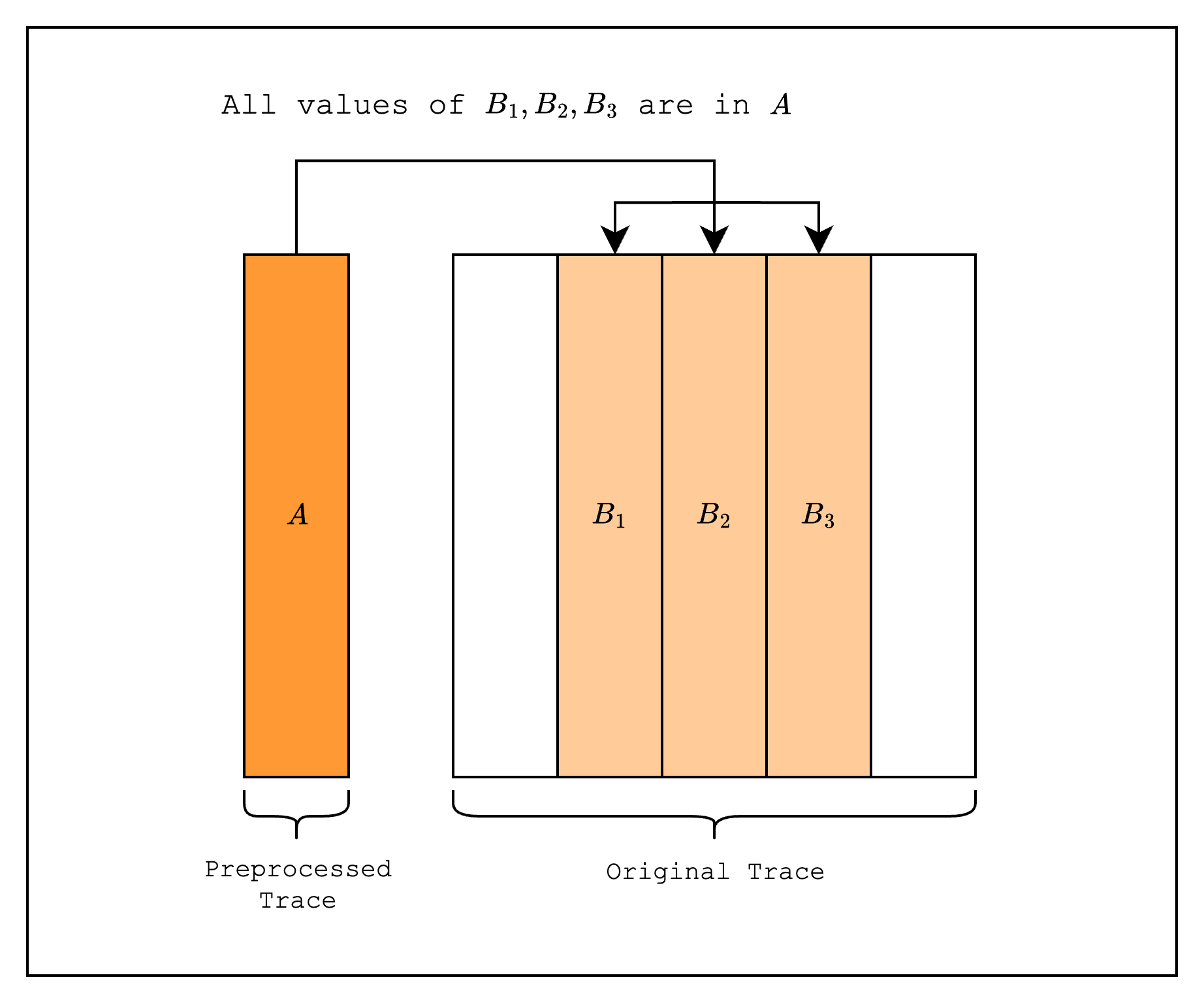
Then, we add a multiplicity column to the original trace indicating the number of times each value in appears in the original trace.
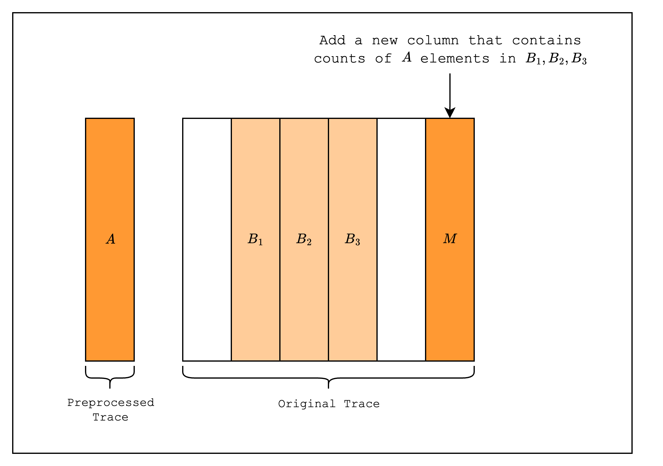
Next, we create LogUp columns as part of the interaction trace, one for the preprocessed trace and the multiplicity column, and another for the batch of all lookups.
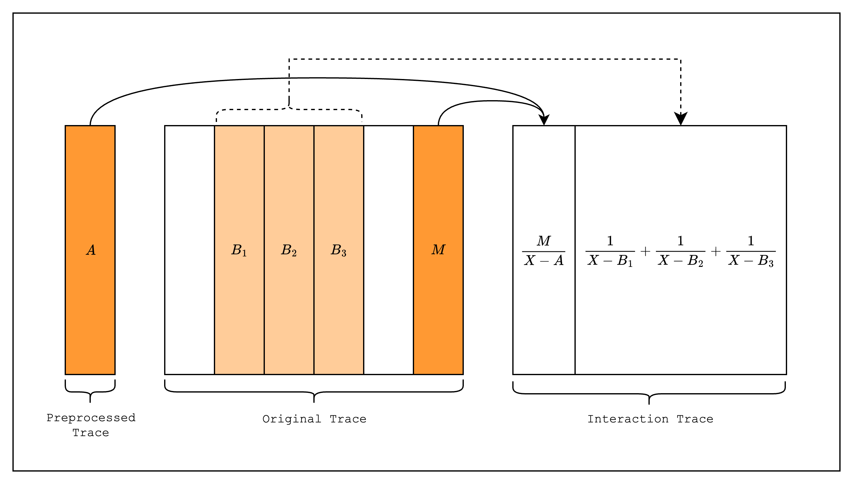
To create a constraint over the LogUp columns, Stwo modifies the LogUp columns to contain the cumulative sum of the fractions in each row. This results in columns that look like the following:
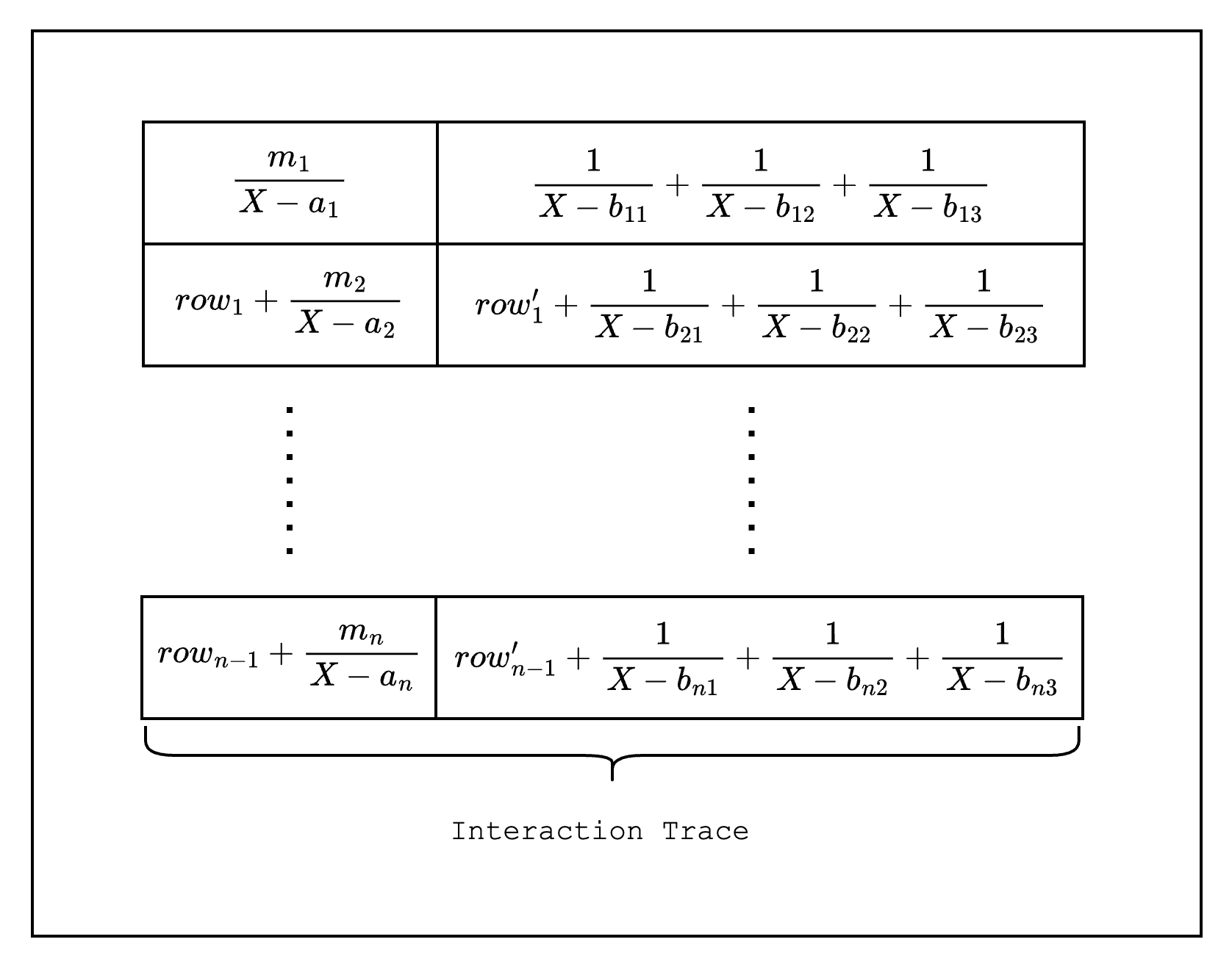
A constraint is created using the values of two rows of the cumulative sum LogUp column. For example, as in Figure 5, we can create a constraint by subtracting from and checking that it equals the LogUp fraction created using values and :
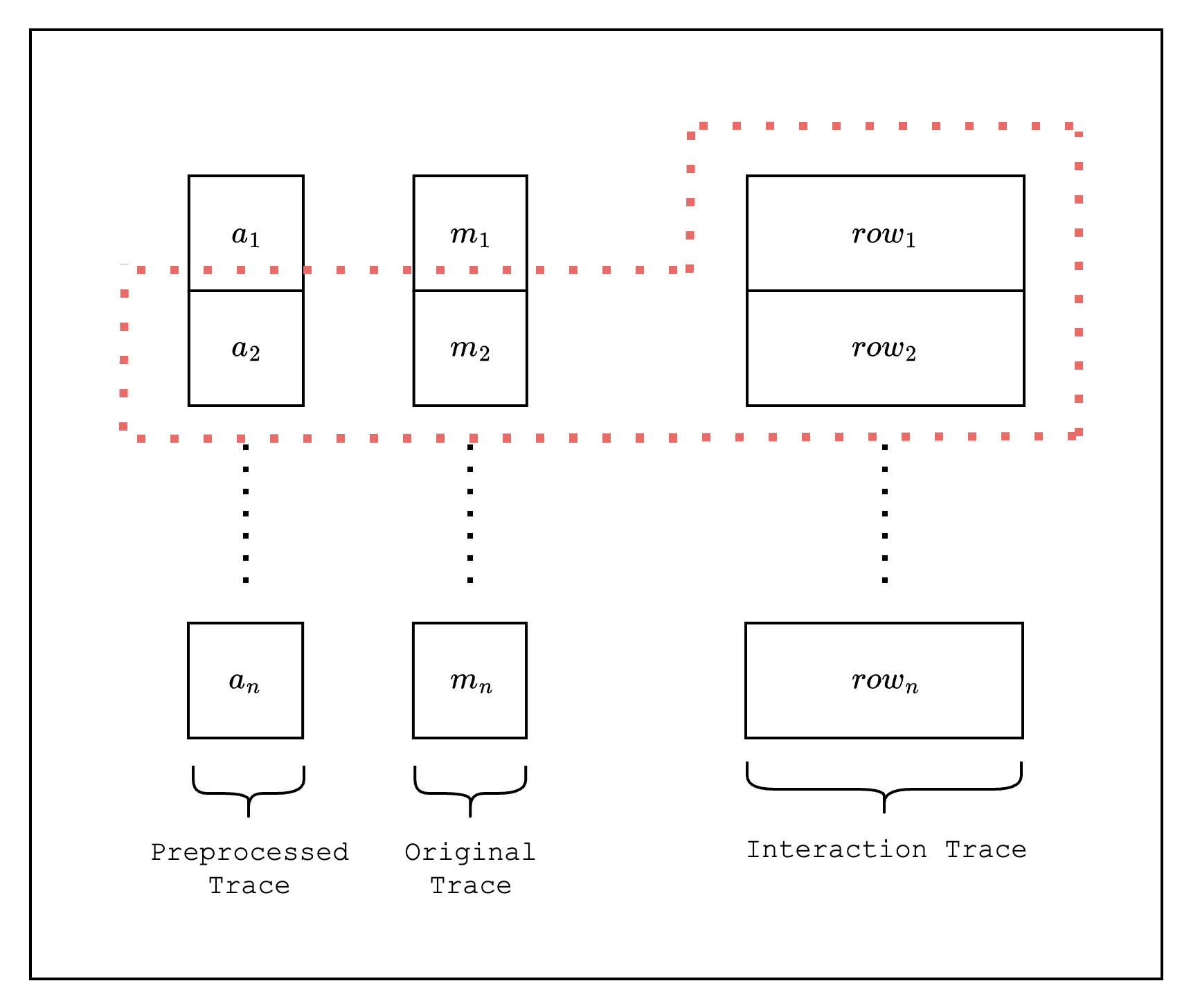
However, this constraint actually does not hold for the first row since . A typical solution to this problem would be to disable this constraint for the first row and create a separate constraint that is enabled only on the first row.
But Stwo solves this problem differently. First, before we accumulate the original LogUp column rows, we subtract each row by the average of the total sum of the rows. Only then do we accumulate each row. This way, the last row of the column will always equal zero, so we do not need to make an exception for the first row. The final constraint for the second row looks as follows:
Where is a witness value provided by the prover.
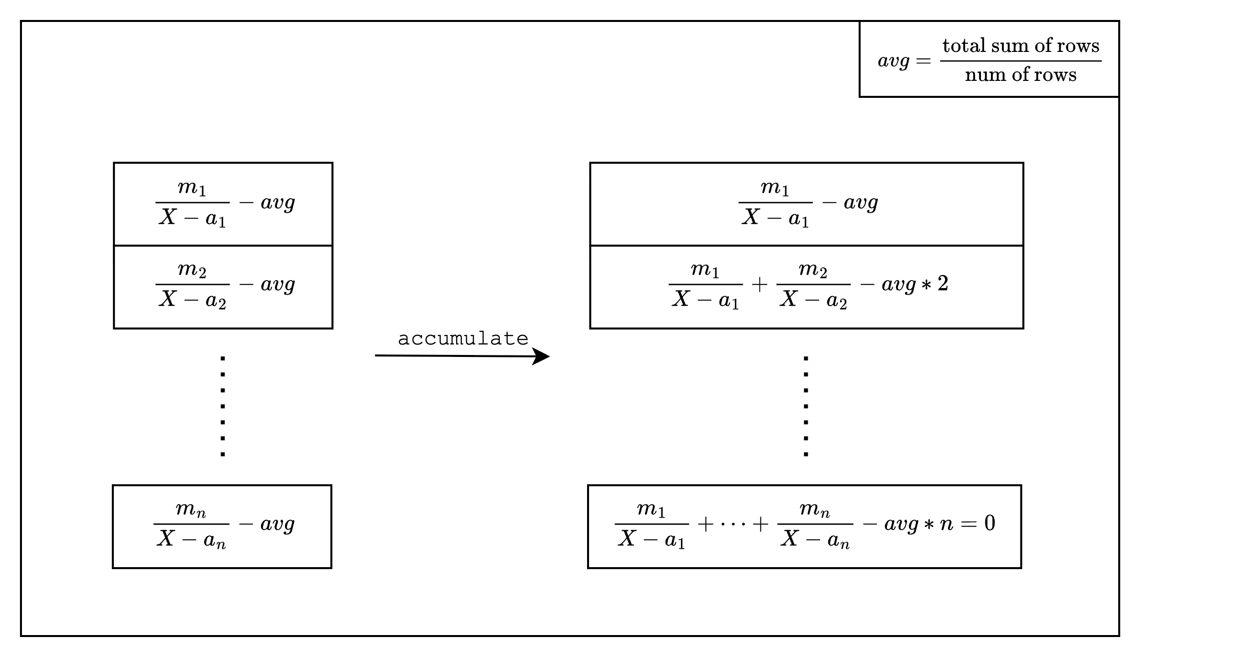
The right column in Figure 6 is the final form of the LogUp column that Stwo commits to as part of the interaction trace.
Batching
In general, batching multiple lookups together helps reduce the size of the proof as it reduces the number of LogUp columns, which means we can commit to fewer columns. However, we cannot batch an arbitrary number of fractions together because it increases the degree of the constraint polynomial.
More specifically, the degree of the constraint polynomial increases linearly with the number of fractions in the batch. Let's say we want to batch fractions together. This will create a constraint . Once we multiply both sides by the common denominator, we get a constraint of degree from the product .
To illustrate the accounting for how many fractions we can batch together, we first need to understand how the degree of the composition polynomial is calculated in Stwo. Here, the composition polynomial is the constraint polynomial divided by the quotient polynomial, where the quotient polynomial is the vanishing polynomial of the trace domain (i.e. evaluates to 0 over the trace domain). So let's say we have a degree- constraint on two columns: . We can define the composition polynomial as where is the trace height. The degree of and is so, if the constraint holds, the degree of the composition polynomial is . Thus, given that we already has evaluations, we can expand it by to convince the verifier that the constraint holds since .
Now, coming back to the question of how many fractions we can batch together, we can see that we can batch up to exactly fractions if the rate of expansion is .
Awesome Stwo
We refer you to the Awesome Stwo repo for additional resources on Stwo and a list of awesome projects building on Stwo.
Benchmarks Report
- Overview of zkVM and Proof Systems
| zkVM / Proof System | Architecture | Frontend | Backend | Security Bits |
|---|---|---|---|---|
| RISC Zero | RISC-V | Rust | STARK-based | 96 bits |
| SP1 | RISC-V | Rust | STARK-based | 100 bits |
| OpenVM | RISC-V | Rust | STARK-based | 100 bits |
| Jolt | RISC-V | Rust | Lookup-based | - |
| Stone | Cairo VM | Cairo | STARK-based | 100 bits |
| Stwo | Cairo VM | Cairo | STARK-based | 96 bits |
- All benchmarks presented here are CPU-only and do not utilize any GPU acceleration.
- Stone benchmarks were generated using the
dynamiclayout with these configurations. - The benchmarks for SP1, R0 and OpenVM use compressed or succinct prover type, which aggregates all the STARK proofs into a single STARK proof.
- Benchmarks which run out of memory have been indicated by
💾and benchmarks which generate errors in proof generation have been indicated by❌in the tables.
Time and Commit Hash
- Commit Hash: f27856ec17fbd9e85ec31cba9c2cb9e96d8dd08f
- Timestamp: Thursday, July 03, 2025 20:52:50 UTC
System Information
OS Version
Ubuntu 24.04.2 LTS
CPU Info
-
Architecture: x86_64
-
CPU(s): 48
-
Model name: AMD EPYC-Rome Processor
-
Thread(s) per core: 2
-
Core(s) per socket: 24
-
Socket(s): 1
-
L3 cache: 16 MiB (1 instance)
Memory Info
-
MemTotal: 184.25 GB
-
MemFree: 166.19 GB
-
MemAvailable: 178.69 GB
Fibonacci
Benchmark n Fibonacci iterations.
Prover Time (s)
| n | jolt | sp1 | openvm | r0 | stone | stwo |
|---|---|---|---|---|---|---|
| 32768 | 3.208 | 15.003 | 34.291 | 17.128 | 56.325 | 13.198 |
| 65536 | 5.183 | 18.252 | 42.403 | 29.241 | 95.468 | 11.372 |
| 131072 | 9.17 | 24.982 | 57.978 | 52.298 | 💾 | 12.886 |
| 262144 | 15.771 | 39.327 | 92.229 | 86.743 | 💾 | 12.587 |
| 524288 | 28.16 | 54.812 | 158.128 | 167.607 | 💾 | 16.166 |
| 1048576 | 54.42 | 72.028 | 320.082 | 306.386 | 💾 | 18.612 |
| 2097152 | 107.89 | 128.215 | 515.567 | 605.92 | 💾 | 31.047 |
| 4194304 | ❌ | 222.332 | 1042.58 | 1206.76 | 💾 | 60.939 |
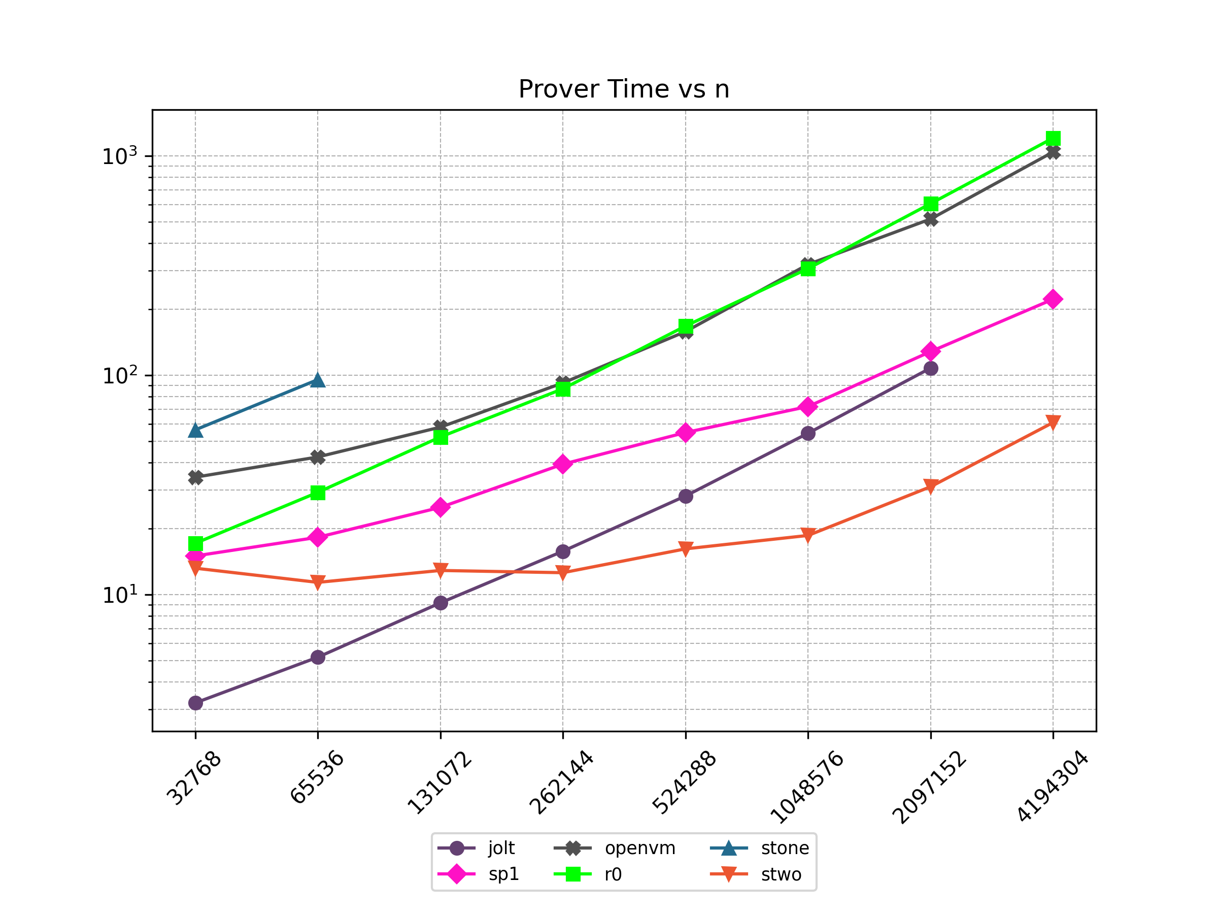
Verifier Time (ms)
| n | jolt | sp1 | openvm | r0 | stone | stwo |
|---|---|---|---|---|---|---|
| 32768 | 53.0 | 108 | 142 | 23 | 92.0 | 41 |
| 65536 | 77.0 | 107 | 139 | 10 | 113.0 | 16 |
| 131072 | 58.0 | 101 | 140 | 23 | 💾 | 18 |
| 262144 | 103.0 | 100 | 141 | 22 | 💾 | 89 |
| 524288 | 56.0 | 83 | 140 | 24 | 💾 | 14 |
| 1048576 | 104.0 | 83 | 57 | 23 | 💾 | 414 |
| 2097152 | 98.0 | 84 | 57 | 10 | 💾 | 367 |
| 4194304 | ❌ | 83 | 57 | 23 | 💾 | 10 |
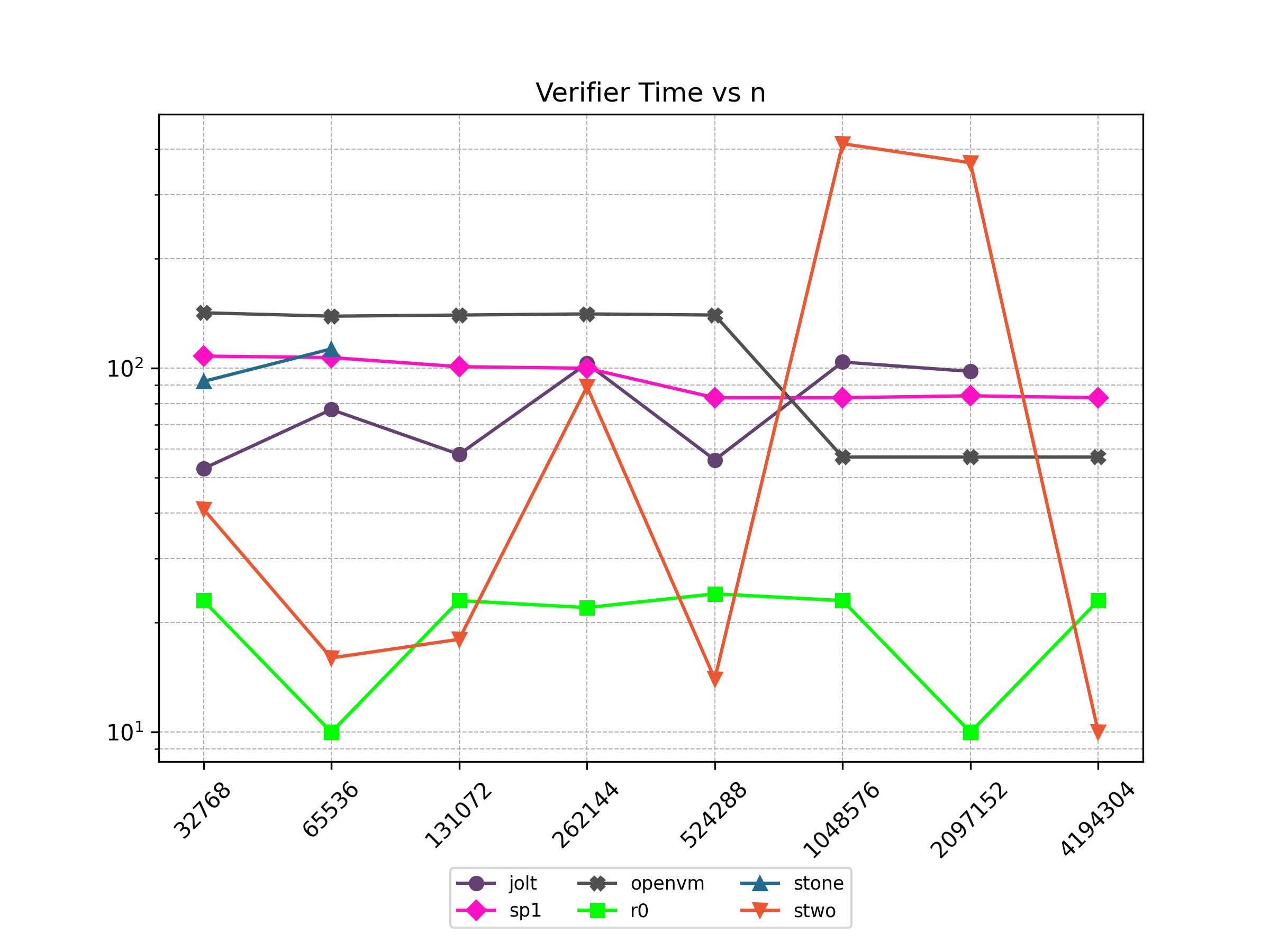
Proof Size (KB)
| n | jolt | sp1 | openvm | r0 | stone | stwo |
|---|---|---|---|---|---|---|
| 32768 | 187.615 | 1315.53 | 1708.31 | 223.234 | 125.608 | 789.578 |
| 65536 | 197.799 | 1315.53 | 1708.31 | 223.234 | 129.8 | 783.63 |
| 131072 | 208.399 | 1315.53 | 1708.31 | 223.234 | 💾 | 783.834 |
| 262144 | 219.415 | 1315.53 | 1708.31 | 223.234 | 💾 | 802.678 |
| 524288 | 230.847 | 1315.53 | 1708.31 | 223.234 | 💾 | 801.194 |
| 1048576 | 242.695 | 1315.53 | 852.937 | 223.234 | 💾 | 808.038 |
| 2097152 | 254.959 | 1315.53 | 852.937 | 223.234 | 💾 | 819.122 |
| 4194304 | ❌ | 1315.53 | 816.649 | 223.234 | 💾 | 866.882 |
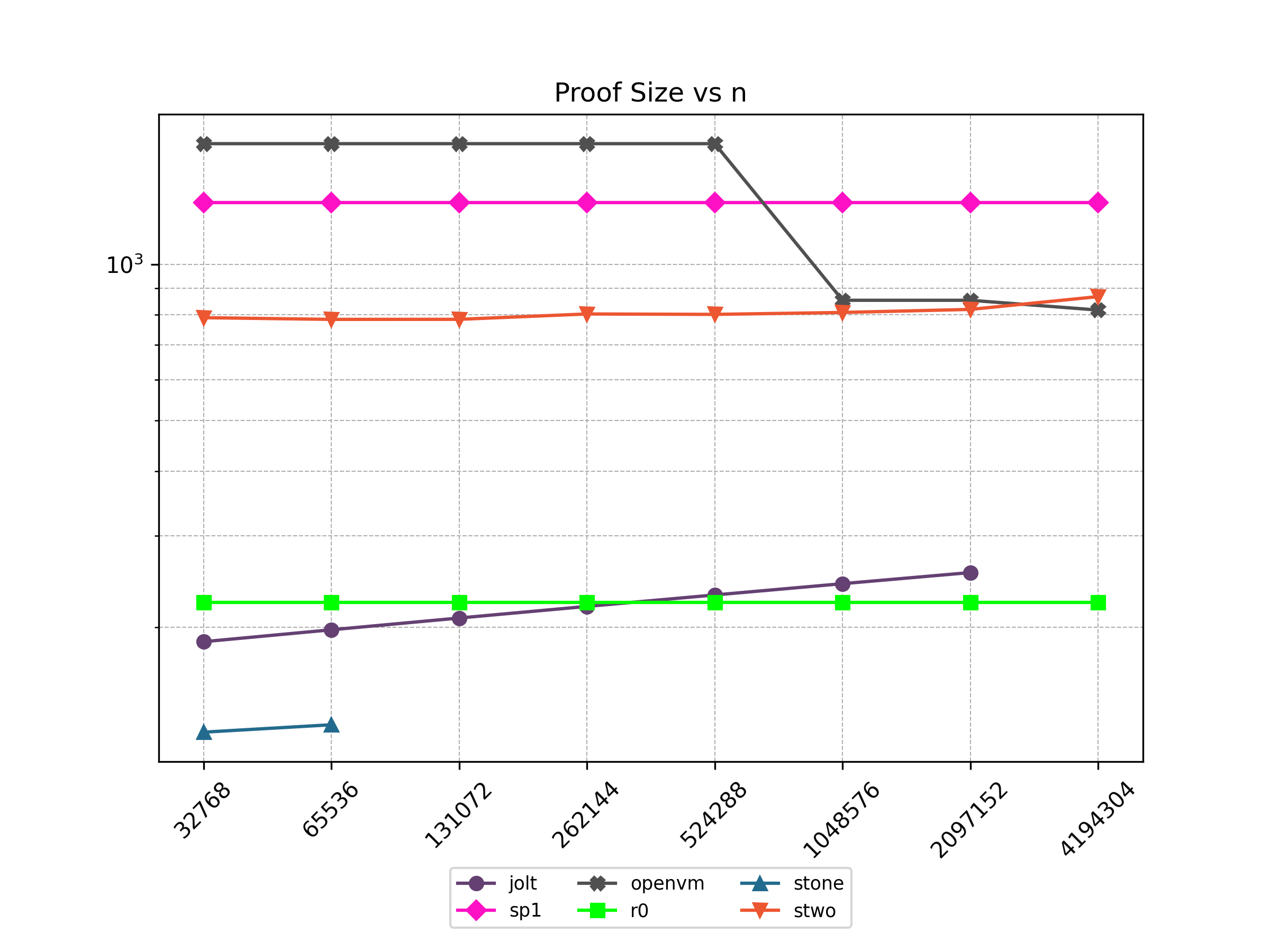
Cycle Count
| n | jolt | sp1 | r0 | stone | stwo |
|---|---|---|---|---|---|
| 32768 | 196974 | 168808 | 166215 | 229390 | 262143 |
| 65536 | 393582 | 332648 | 330055 | 458766 | 524287 |
| 131072 | 786798 | 660328 | 657735 | 💾 | 1048575 |
| 262144 | 1573230 | 1315688 | 1313095 | 💾 | 2097151 |
| 524288 | 3146041 | 2626408 | 2623815 | 💾 | 4194303 |
| 1048576 | 6291822 | 5247848 | 5245255 | 💾 | 8388607 |
| 2097152 | 12583293 | 10490728 | 10488135 | 💾 | 16777215 |
| 4194304 | ❌ | 20976488 | 20973895 | 💾 | 33554431 |
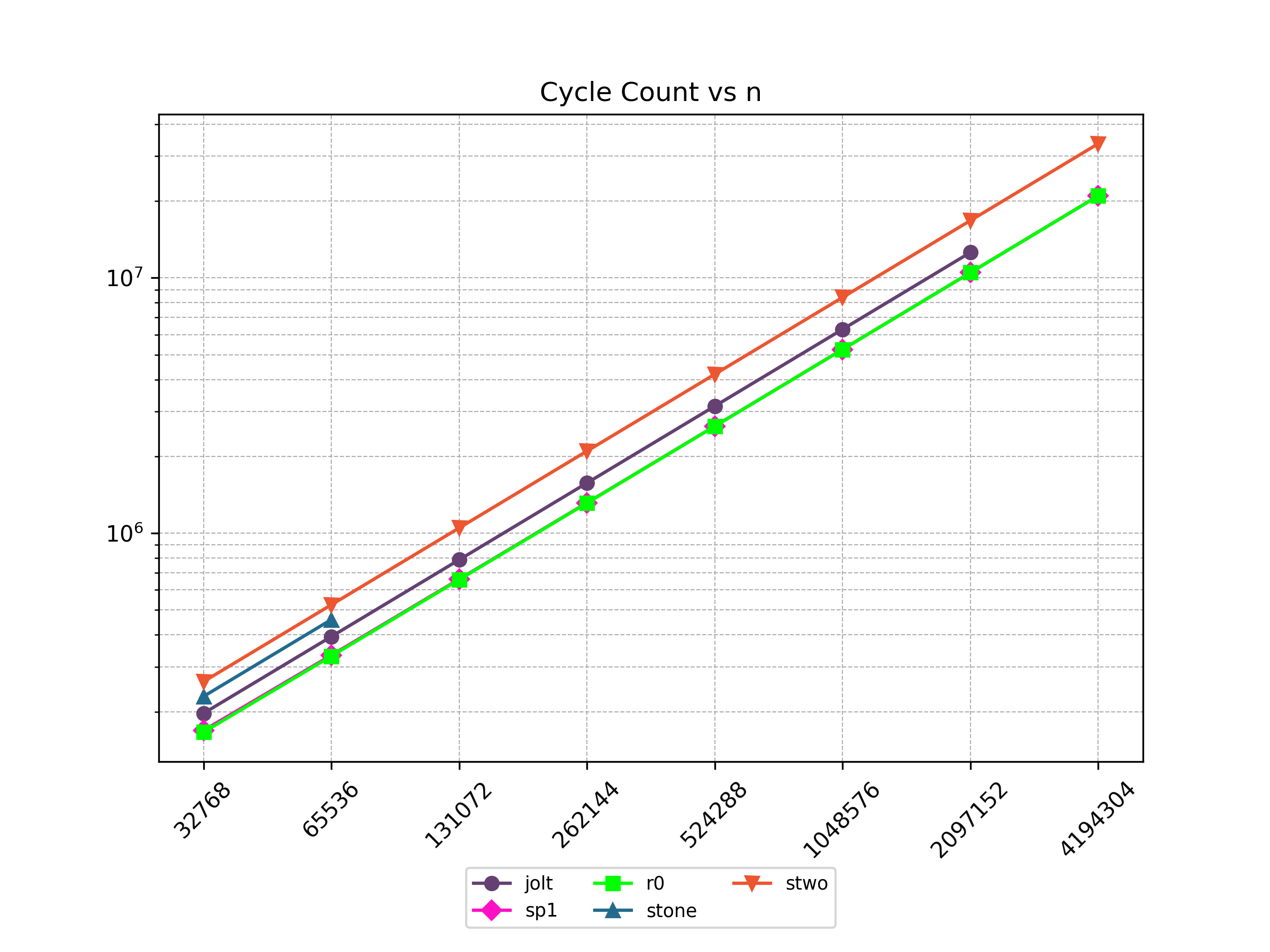
Peak Memory (GB)
| n | jolt | sp1 | openvm | r0 | stone | stwo |
|---|---|---|---|---|---|---|
| 32768 | 6.44 | 5.12 | 7 | 2.3 | 59.44 | 11.08 |
| 65536 | 5.83 | 6.42 | 5.43 | 4.58 | 118.54 | 11.46 |
| 131072 | 8.79 | 9.18 | 5.43 | 9.15 | 💾 | 12.2 |
| 262144 | 14.73 | 14.3 | 6.57 | 9.17 | 💾 | 14.01 |
| 524288 | 26.95 | 15.12 | 12.22 | 9.17 | 💾 | 17.57 |
| 1048576 | 50.85 | 25.94 | 12.22 | 9.17 | 💾 | 24.57 |
| 2097152 | 98.93 | 35.61 | 12.42 | 9.18 | 💾 | 38.62 |
| 4194304 | ❌ | 51.25 | 12.43 | 9.18 | 💾 | 72.26 |
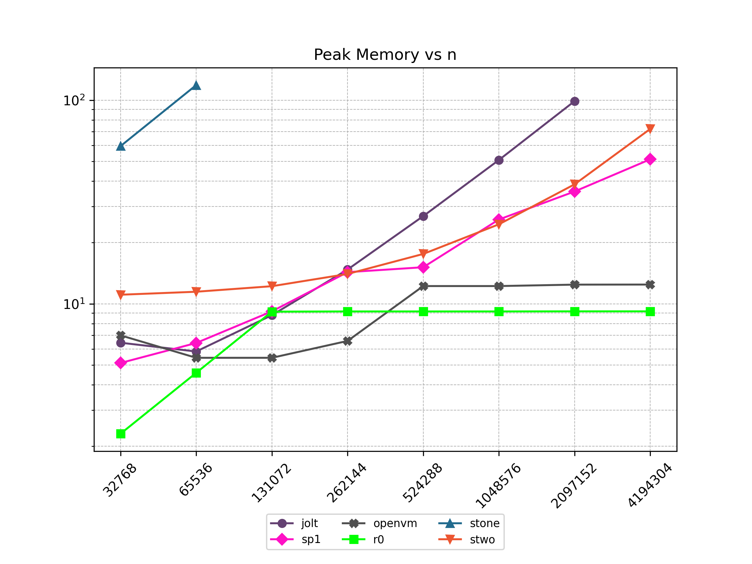
Sha2
Benchmark Sha256 hash of n bytes. For Stone, the cairo implementation of sha256 by cartridge was used for benchmarking and for other zkvms sha2 Rust crate was used for benchmarking.
Prover Time (s)
| n | jolt | sp1 | openvm | r0 | stone | stwo | sp1-precompile | r0-precompile | openvm-precompile |
|---|---|---|---|---|---|---|---|---|---|
| 256 | 1.657 | 12.71 | 28.943 | 11.196 | 10.835 | 17.978 | 34.019 | 8.316 | 44.301 |
| 512 | 1.711 | 13.184 | 29.561 | 11.306 | 19.88 | 15.051 | 33.991 | 11.33 | 43.728 |
| 1024 | 2.173 | 13.863 | 30.609 | 17.136 | 31.021 | 16.833 | 33.83 | 11.201 | 44.897 |
| 2048 | 3.324 | 15.021 | 34.184 | 28.934 | 31.294 | 17.726 | 34.531 | 17.174 | 44.683 |
| 4096 | ❌ | 16.88 | 39.38 | 52.487 | 66.539 | 14.084 | 34.418 | 28.982 | 47.701 |
| 8192 | ❌ | 24.037 | 50.539 | 86.688 | 116.467 | 14.979 | 35.564 | 52.48 | 48.995 |
| 16384 | ❌ | 37.958 | 78.057 | 167.856 | 💾 | 21.402 | 38.267 | 110.887 | 52.865 |
| 32768 | ❌ | 52.566 | 129.842 | 300.572 | 💾 | 16.555 | 46.209 | 184.873 | 60.148 |
| 65536 | ❌ | 72.136 | 249.403 | 589.84 | 💾 | 18.384 | 60.138 | 357.716 | 79.957 |
| 131072 | ❌ | 136.592 | 532.796 | 1172.21 | 💾 | 27.871 | 87.29 | 709.726 | 124.996 |
| 262144 | ❌ | 257.02 | 916.603 | 2338.03 | 💾 | 27.362 | 121.022 | 1415.34 | 219.654 |
| 524288 | ❌ | 513.726 | 1790.29 | 4673.32 | 💾 | 43.242 | 233.959 | 2825.46 | 393.678 |
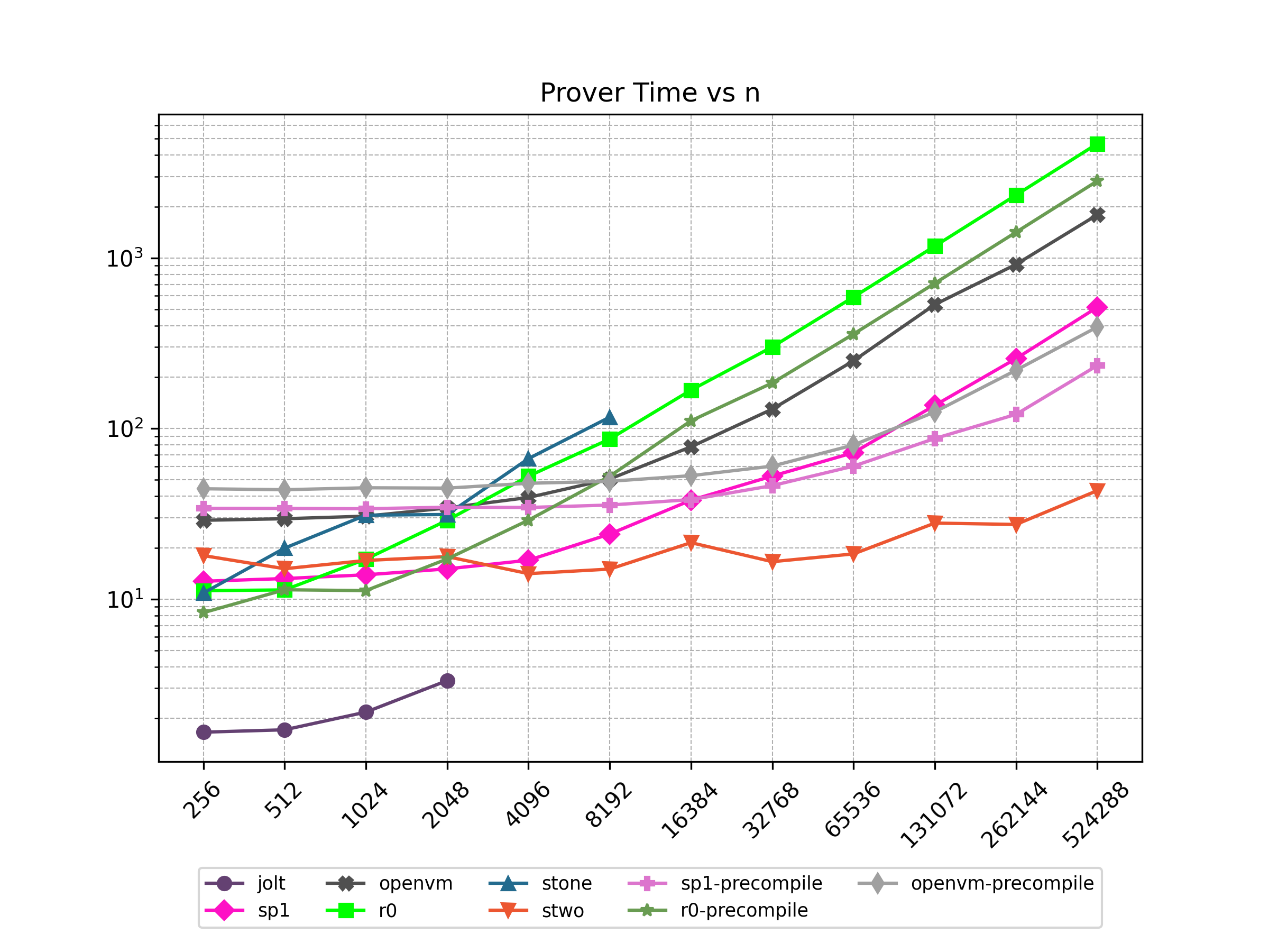
Verifier Time (ms)
| n | jolt | sp1 | openvm | r0 | stone | stwo | sp1-precompile | r0-precompile | openvm-precompile |
|---|---|---|---|---|---|---|---|---|---|
| 256 | 50.0 | 108 | 141 | 10 | 428.0 | 10 | 83 | 22 | 142 |
| 512 | 49.0 | 113 | 144 | 20 | 418.0 | 11 | 106 | 23 | 141 |
| 1024 | 49.0 | 102 | 140 | 23 | 426.0 | 11 | 90 | 15 | 141 |
| 2048 | 75.0 | 97 | 140 | 22 | 440.0 | 11 | 109 | 22 | 142 |
| 4096 | ❌ | 106 | 139 | 22 | 454.0 | 11 | 99 | 23 | 141 |
| 8192 | ❌ | 109 | 141 | 22 | 525.0 | 11 | 87 | 22 | 142 |
| 16384 | ❌ | 82 | 144 | 22 | 💾 | 42 | 92 | 23 | 142 |
| 32768 | ❌ | 94 | 140 | 23 | 💾 | 49 | 102 | 15 | 142 |
| 65536 | ❌ | 83 | 141 | 23 | 💾 | 143 | 95 | 23 | 141 |
| 131072 | ❌ | 83 | 57 | 24 | 💾 | 441 | 83 | 24 | 141 |
| 262144 | ❌ | 83 | 56 | 24 | 💾 | 236 | 83 | 23 | 142 |
| 524288 | ❌ | 83 | 56 | 23 | 💾 | 12 | 82 | 24 | 141 |
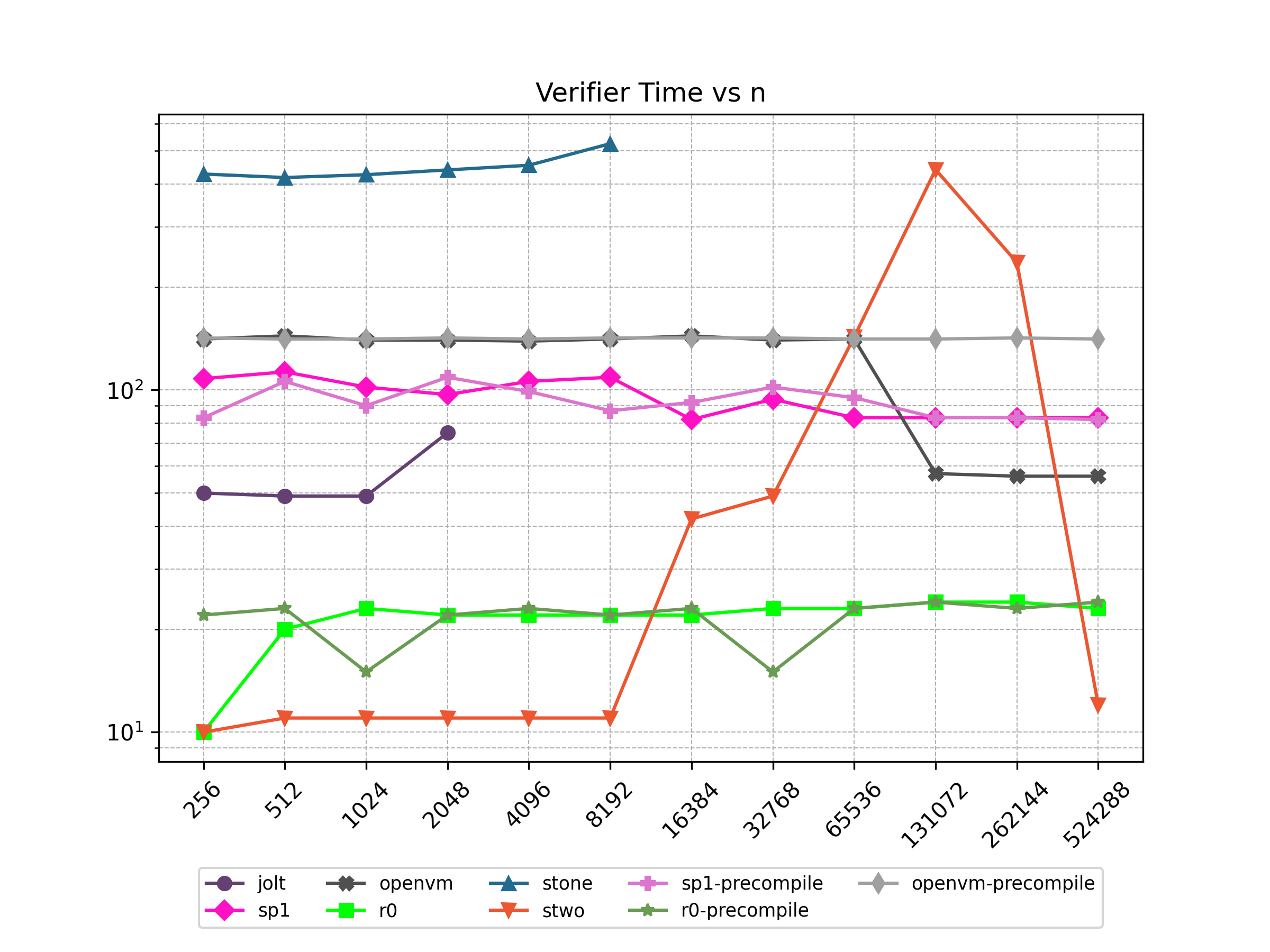
Proof Size (KB)
| n | jolt | sp1 | openvm | r0 | stone | stwo | sp1-precompile | r0-precompile | openvm-precompile |
|---|---|---|---|---|---|---|---|---|---|
| 256 | 172.143 | 1315.56 | 1708.31 | 223.482 | 104.104 | 986.394 | 1315.56 | 223.482 | 1784.35 |
| 512 | 172.143 | 1315.56 | 1708.31 | 223.482 | 114.152 | 1000.61 | 1315.56 | 223.482 | 1784.35 |
| 1024 | 181.495 | 1315.56 | 1708.31 | 223.482 | 117.224 | 1011.16 | 1315.56 | 223.482 | 1784.35 |
| 2048 | 191.263 | 1315.56 | 1708.31 | 223.482 | 120.04 | 1011.71 | 1315.56 | 223.482 | 1784.35 |
| 4096 | ❌ | 1315.56 | 1708.31 | 223.482 | 126.632 | 1007.77 | 1315.56 | 223.482 | 1784.35 |
| 8192 | ❌ | 1315.56 | 1708.31 | 223.482 | 130.824 | 1013.42 | 1315.56 | 223.482 | 1784.35 |
| 16384 | ❌ | 1315.56 | 1708.31 | 223.482 | 💾 | 1005.31 | 1315.56 | 223.482 | 1784.35 |
| 32768 | ❌ | 1315.56 | 1708.31 | 223.482 | 💾 | 1018.49 | 1315.56 | 223.482 | 1784.35 |
| 65536 | ❌ | 1315.56 | 1708.31 | 223.482 | 💾 | 1017.72 | 1315.56 | 223.482 | 1784.35 |
| 131072 | ❌ | 1315.56 | 852.937 | 223.482 | 💾 | 1037.15 | 1315.56 | 223.482 | 1784.35 |
| 262144 | ❌ | 1315.56 | 852.937 | 223.482 | 💾 | 1045.93 | 1315.56 | 223.482 | 1784.35 |
| 524288 | ❌ | 1315.56 | 816.649 | 223.482 | 💾 | 1092.14 | 1315.56 | 223.482 | 1784.35 |
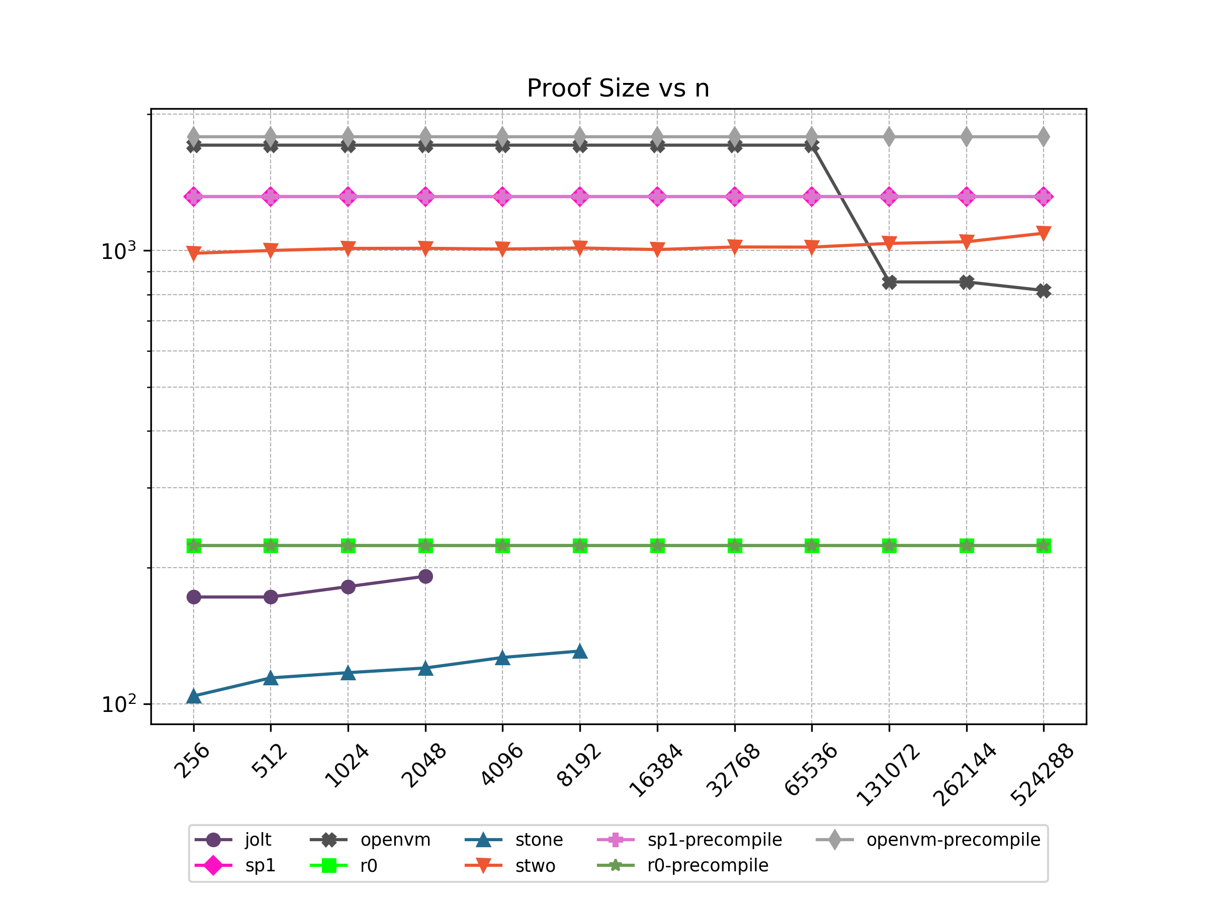
Cycle Count
| n | jolt | sp1 | r0 | stone | stwo | sp1-precompile | r0-precompile |
|---|---|---|---|---|---|---|---|
| 256 | 35325.0 | 33911 | 51280 | 14791.0 | 131071 | 11492 | 31643 |
| 512 | 60893.0 | 52743 | 90848 | 29233.0 | 131071 | 15820 | 55467 |
| 1024 | 112029 | 90407 | 169984 | 46295.0 | 131071 | 24476 | 103133 |
| 2048 | 214301 | 165735 | 328256 | 80419.0 | 131071 | 41788 | 198463 |
| 4096 | ❌ | 316391 | 644800 | 160489 | 262143 | 76412 | 389106 |
| 8192 | ❌ | 617703 | 1277888 | 308807 | 524287 | 145660 | 770392 |
| 16384 | ❌ | 1220327 | 2544064 | 💾 | 1048575 | 284156 | 1532981 |
| 32768 | ❌ | 2425575 | 5076416 | 💾 | 2097151 | 561148 | 3058159 |
| 65536 | ❌ | 4836071 | 10141120 | 💾 | 4194303 | 1115132 | 6108532 |
| 131072 | ❌ | 9657063 | 20270528 | 💾 | 8388607 | 2223100 | 12209241 |
| 262144 | ❌ | 19299047 | 40529344 | 💾 | 16777215 | 4439036 | 24410676 |
| 524288 | ❌ | 38583015 | 81046976 | 💾 | 33554431 | 8870908 | 48813546 |
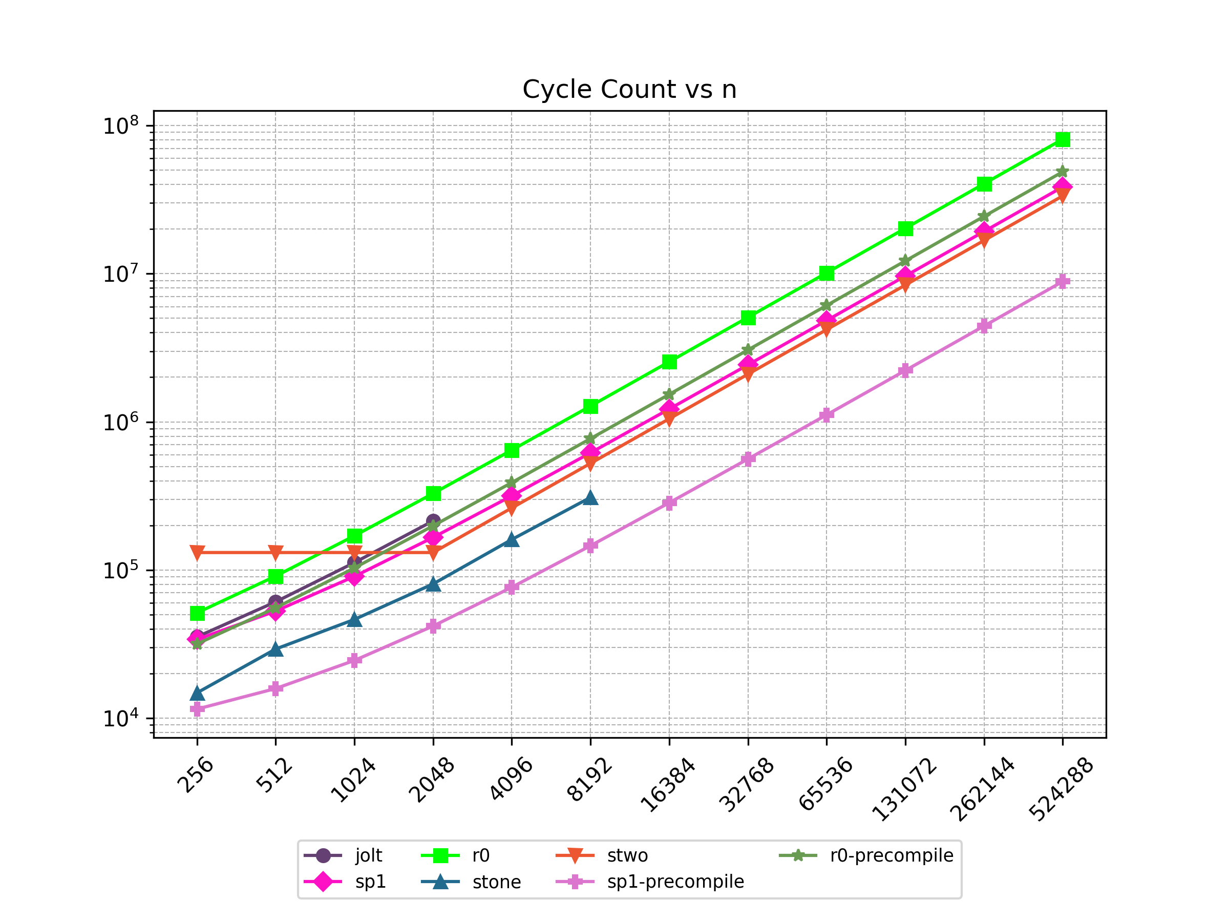
Peak Memory (GB)
| n | jolt | sp1 | openvm | r0 | stone | stwo | sp1-precompile | r0-precompile | openvm-precompile |
|---|---|---|---|---|---|---|---|---|---|
| 256 | 5.09 | 4.29 | 5.45 | 1.43 | 9.63 | 10.79 | 7.84 | 1.43 | 5.44 |
| 512 | 4.9 | 4.42 | 5.44 | 1.42 | 18.9 | 10.82 | 8.18 | 1.42 | 5.45 |
| 1024 | 4.9 | 4.54 | 5.44 | 2.3 | 35.74 | 10.86 | 8.01 | 1.42 | 5.44 |
| 2048 | 4.91 | 5.02 | 5.44 | 4.58 | 35.73 | 10.87 | 8.1 | 2.3 | 5.44 |
| 4096 | ❌ | 6.28 | 5.44 | 9.15 | 71.46 | 11.03 | 8.29 | 4.59 | 5.44 |
| 8192 | ❌ | 8.6 | 5.44 | 9.17 | 142.68 | 11.34 | 8.53 | 9.16 | 5.44 |
| 16384 | ❌ | 13.32 | 5.44 | 9.18 | 💾 | 11.94 | 8.79 | 9.17 | 5.44 |
| 32768 | ❌ | 15.31 | 8.78 | 9.18 | 💾 | 13.48 | 8.63 | 9.18 | 5.44 |
| 65536 | ❌ | 29.19 | 16.64 | 9.18 | 💾 | 16.52 | 12.9 | 9.18 | 5.44 |
| 131072 | ❌ | 35.4 | 21.6 | 9.2 | 💾 | 22.5 | 21.26 | 9.19 | 6.89 |
| 262144 | ❌ | 45.34 | 22.77 | 9.21 | 💾 | 34.52 | 34.15 | 9.21 | 12.86 |
| 524288 | ❌ | 54.88 | 25.59 | 9.25 | 💾 | 63.89 | 49.57 | 9.23 | 24.78 |
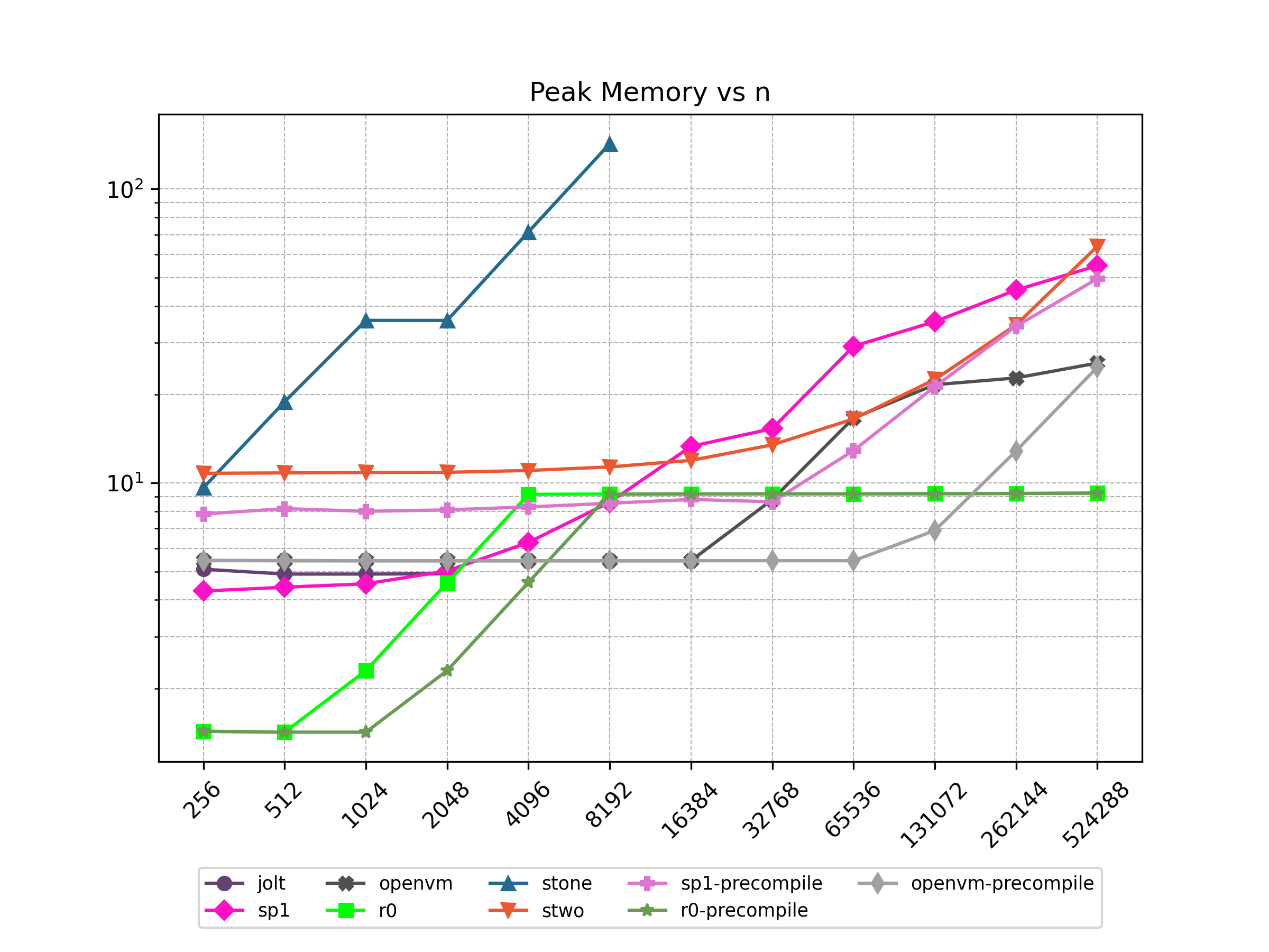
Sha2-Chain
Benchmark Sha256 hash of 32 bytes for n iteration.
Prover Time (s)
| n | jolt | sp1 | openvm | r0 | stone | stwo | sp1-precompile | r0-precompile | openvm-precompile |
|---|---|---|---|---|---|---|---|---|---|
| 8 | 2.164 | 12.798 | 29.444 | 11.303 | 11.083 | 11.488 | 34.606 | 6.862 | 43.511 |
| 16 | 2.973 | 13.875 | 30.349 | 11.252 | 11.115 | 18.583 | 34.339 | 8.352 | 44.295 |
| 32 | 4.912 | 14.62 | 33.814 | 17.156 | 11.991 | 11.938 | 34.203 | 8.305 | 43.893 |
| 64 | 8.285 | 17.617 | 38.294 | 28.948 | 10.631 | 14.158 | 33.862 | 11.289 | 44.197 |
| 128 | 14.469 | 24.728 | 49.582 | 52.457 | 19.206 | 10.335 | 35.134 | 11.315 | 45.006 |
| 256 | 25.909 | 37.471 | 73.574 | 74.818 | 26.184 | 14.057 | 36.234 | 17.422 | 42.793 |
| 512 | 50.064 | 52.895 | 126.086 | 144.234 | 56.529 | 22.012 | 40.643 | 29.057 | 46.573 |
| 1024 | 96.901 | 71.752 | 231.888 | 285.012 | 95.878 | 20.846 | 50.02 | 52.522 | 52.862 |
| 2048 | ❌ | 132.275 | 516.789 | 574.819 | 💾 | 14.061 | 77.808 | 110.071 | 61.761 |
| 4096 | ❌ | 227.325 | 905.706 | 1110.77 | 💾 | 17.799 | 103.011 | 191.208 | 81.617 |
| 8192 | ❌ | 444.028 | 1814.44 | 2210.89 | 💾 | 18.607 | 193.572 | 365.446 | 122.31 |
| 16384 | ❌ | 872.638 | 3596.93 | 4404.24 | 💾 | 20.569 | 319.33 | 723.963 | 212.16 |
| 32768 | ❌ | 1698.85 | 7067.26 | 8791.74 | 💾 | 25.041 | 628.712 | 1443.04 | 388.56 |
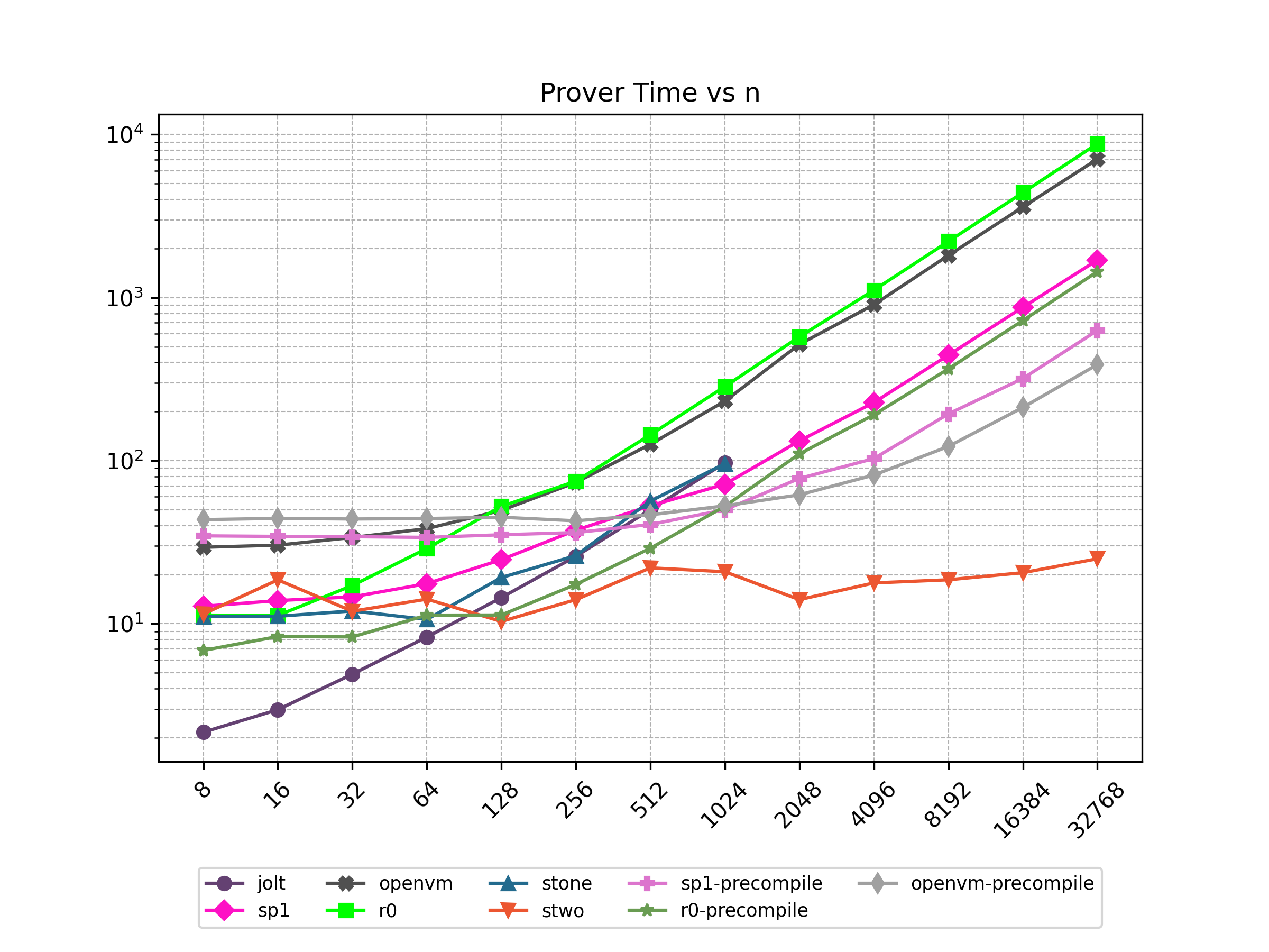
Verifier Time (ms)
| n | jolt | sp1 | openvm | r0 | stone | stwo | sp1-precompile | r0-precompile | openvm-precompile |
|---|---|---|---|---|---|---|---|---|---|
| 8 | 49.0 | 82 | 140 | 22 | 432.0 | 10 | 83 | 23 | 141 |
| 16 | 55.0 | 101 | 140 | 23 | 398.0 | 10 | 93 | 20 | 142 |
| 32 | 86.0 | 108 | 140 | 22 | 402.0 | 10 | 94 | 21 | 141 |
| 64 | 102.0 | 88 | 140 | 23 | 375.0 | 10 | 87 | 22 | 141 |
| 128 | 78.0 | 108 | 141 | 23 | 413.0 | 10 | 84 | 21 | 141 |
| 256 | 60.0 | 83 | 139 | 22 | 422.0 | 11 | 83 | 23 | 141 |
| 512 | 60.0 | 84 | 140 | 22 | 420.0 | 37 | 83 | 22 | 142 |
| 1024 | 103.0 | 83 | 139 | 23 | 456.0 | 41 | 83 | 22 | 141 |
| 2048 | ❌ | 83 | 57 | 23 | 💾 | 40 | 83 | 10 | 141 |
| 4096 | ❌ | 86 | 56 | 22 | 💾 | 119 | 83 | 23 | 141 |
| 8192 | ❌ | 83 | 56 | 22 | 💾 | 116 | 83 | 10 | 142 |
| 16384 | ❌ | 84 | 56 | 24 | 💾 | 182 | 86 | 23 | 141 |
| 32768 | ❌ | 83 | 56 | 24 | 💾 | 262 | 83 | 23 | 141 |
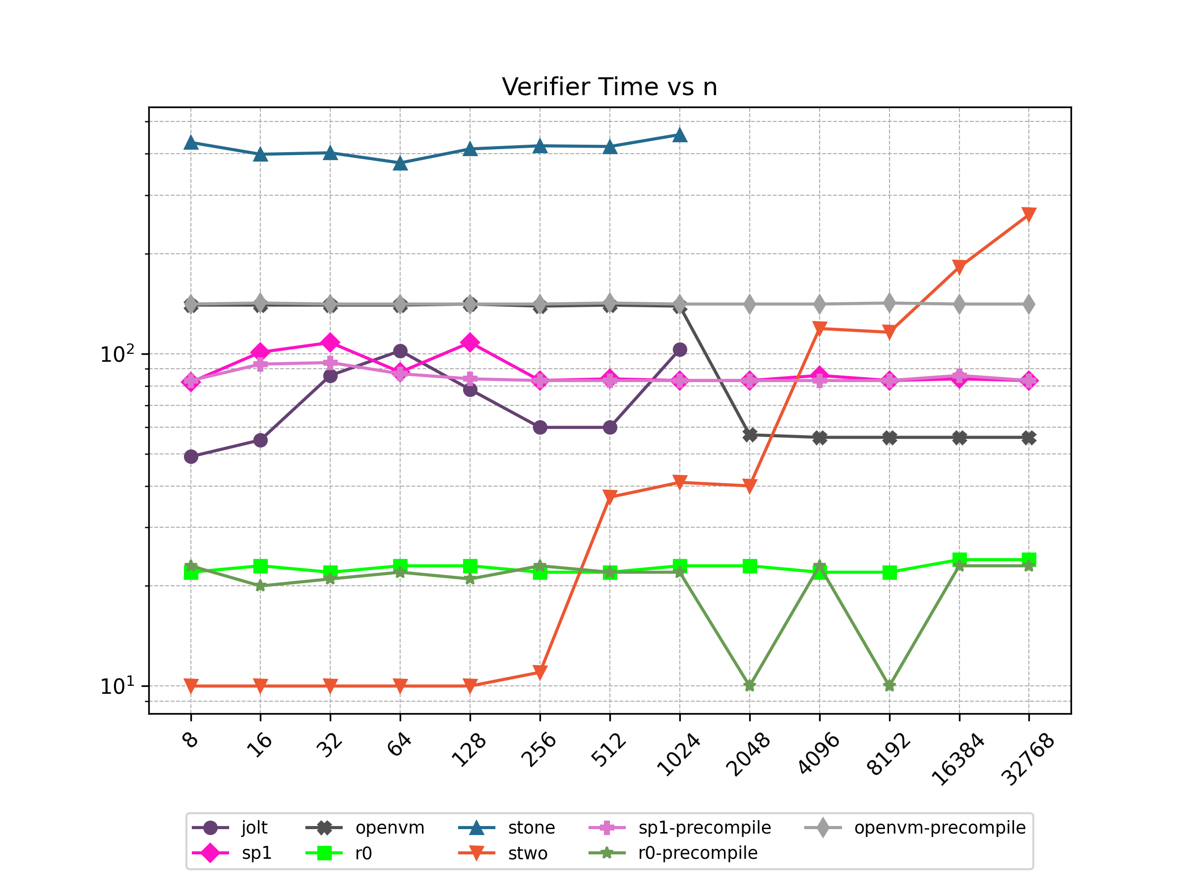
Proof Size (KB)
| n | jolt | sp1 | openvm | r0 | stone | stwo | sp1-precompile | r0-precompile | openvm-precompile |
|---|---|---|---|---|---|---|---|---|---|
| 8 | 181.495 | 1315.56 | 1708.31 | 223.482 | 109.544 | 952.094 | 1315.56 | 223.482 | 1784.35 |
| 16 | 191.263 | 1315.56 | 1708.31 | 223.482 | 106.728 | 971.154 | 1315.56 | 223.482 | 1784.35 |
| 32 | 201.447 | 1315.56 | 1708.31 | 223.482 | 108.776 | 955.554 | 1315.56 | 223.482 | 1784.35 |
| 64 | 212.047 | 1315.56 | 1708.31 | 223.482 | 106.568 | 962.798 | 1315.56 | 223.482 | 1784.35 |
| 128 | 223.063 | 1315.56 | 1708.31 | 223.482 | 112.36 | 946.158 | 1315.56 | 223.482 | 1784.35 |
| 256 | 234.495 | 1315.56 | 1708.31 | 223.482 | 117.992 | 969.698 | 1315.56 | 223.482 | 1784.35 |
| 512 | 246.343 | 1315.56 | 1708.31 | 223.482 | 124.168 | 947.738 | 1315.56 | 223.482 | 1784.35 |
| 1024 | 258.607 | 1315.56 | 1708.31 | 223.482 | 129.512 | 948.874 | 1315.56 | 223.482 | 1784.35 |
| 2048 | ❌ | 1315.56 | 852.937 | 223.482 | 💾 | 959.414 | 1315.56 | 223.482 | 1784.35 |
| 4096 | ❌ | 1315.56 | 852.937 | 223.482 | 💾 | 966.074 | 1315.56 | 223.482 | 1784.35 |
| 8192 | ❌ | 1315.56 | 816.649 | 223.482 | 💾 | 976.142 | 1315.56 | 223.482 | 1784.35 |
| 16384 | ❌ | 1315.56 | 816.649 | 223.482 | 💾 | 986.186 | 1315.56 | 223.482 | 1784.35 |
| 32768 | ❌ | 1315.56 | 852.937 | 223.482 | 💾 | 1001.51 | 1315.56 | 223.482 | 1784.35 |
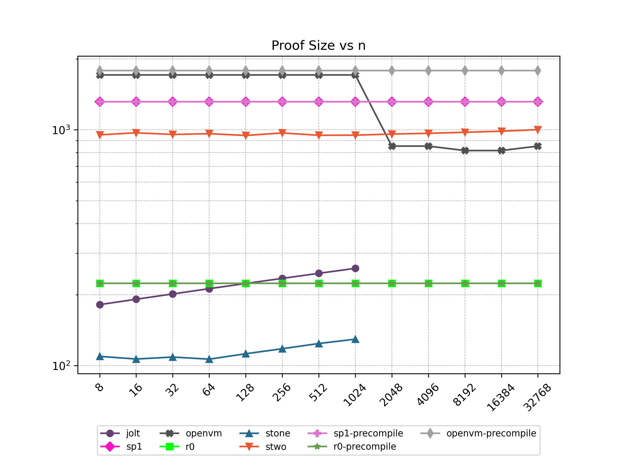
Cycle Count
| n | jolt | sp1 | r0 | stone | stwo | sp1-precompile | r0-precompile |
|---|---|---|---|---|---|---|---|
| 8 | 69290.0 | 48118 | 45952 | 3008.0 | 65535 | 13495 | 14624 |
| 16 | 136282 | 85686 | 83432 | 5872.0 | 65535 | 20287 | 20776 |
| 32 | 270266 | 160822 | 158392 | 11600.0 | 65535 | 33871 | 33080 |
| 64 | 538234 | 311094 | 308312 | 23056.0 | 65535 | 61039 | 57688 |
| 128 | 1074187 | 611638 | 608152 | 45968.0 | 65535 | 115375 | 106904 |
| 256 | 2146059 | 1212726 | 1207832 | 91792.0 | 131071 | 224047 | 205336 |
| 512 | 4289803 | 2414902 | 2407192 | 183440 | 262143 | 441391 | 402200 |
| 1024 | 8577291 | 4819254 | 4805912 | 366736 | 524287 | 876079 | 795928 |
| 2048 | ❌ | 9627958 | 9603352 | 💾 | 1048575 | 1745455 | 1583384 |
| 4096 | ❌ | 19245366 | 19198232 | 💾 | 2097151 | 3484207 | 3158296 |
| 8192 | ❌ | 38480182 | 38387992 | 💾 | 4194303 | 6961711 | 6308120 |
| 16384 | ❌ | 76949814 | 76767512 | 💾 | 8388607 | 13916719 | 12607768 |
| 32768 | ❌ | 153889078 | 153526552 | 💾 | 16777215 | 27826735 | 25207064 |
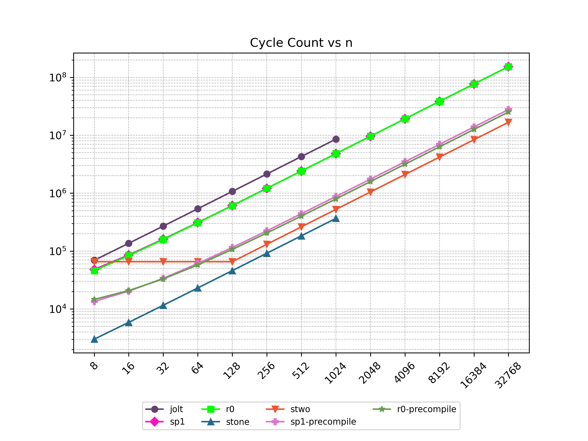
Peak Memory (GB)
| n | jolt | sp1 | openvm | r0 | stone | stwo | sp1-precompile | r0-precompile | openvm-precompile |
|---|---|---|---|---|---|---|---|---|---|
| 8 | 5.1 | 4.31 | 5.44 | 1.42 | 9.1 | 10.74 | 7.81 | 1.44 | 5.44 |
| 16 | 4.91 | 4.54 | 5.44 | 1.42 | 9.04 | 10.74 | 8.04 | 1.43 | 5.44 |
| 32 | 5.92 | 4.98 | 5.44 | 2.3 | 9.04 | 10.75 | 8.5 | 1.43 | 5.44 |
| 64 | 8.69 | 6.19 | 5.44 | 4.58 | 9.05 | 10.77 | 8.05 | 1.42 | 5.44 |
| 128 | 14.39 | 8.81 | 5.44 | 9.14 | 17.87 | 10.78 | 8.29 | 1.42 | 5.44 |
| 256 | 26.36 | 13.27 | 5.44 | 9.17 | 29.66 | 10.83 | 8.52 | 2.3 | 5.44 |
| 512 | 48.32 | 14.7 | 8.57 | 9.17 | 59.33 | 10.95 | 8.63 | 4.59 | 5.44 |
| 1024 | 93.03 | 27.2 | 16.24 | 9.17 | 118.62 | 11.18 | 11.08 | 9.15 | 5.44 |
| 2048 | ❌ | 40.4 | 20.59 | 9.18 | 💾 | 11.64 | 18.61 | 9.17 | 5.44 |
| 4096 | ❌ | 44.04 | 20.6 | 9.19 | 💾 | 12.88 | 35.18 | 9.17 | 5.44 |
| 8192 | ❌ | 55.14 | 20.62 | 9.2 | 💾 | 15.31 | 53.3 | 9.17 | 6.64 |
| 16384 | ❌ | 58.47 | 20.66 | 9.2 | 💾 | 20.08 | 52.23 | 9.18 | 12.34 |
| 32768 | ❌ | 60.22 | 20.8 | 9.27 | 💾 | 29.71 | 63.03 | 9.18 | 23.74 |
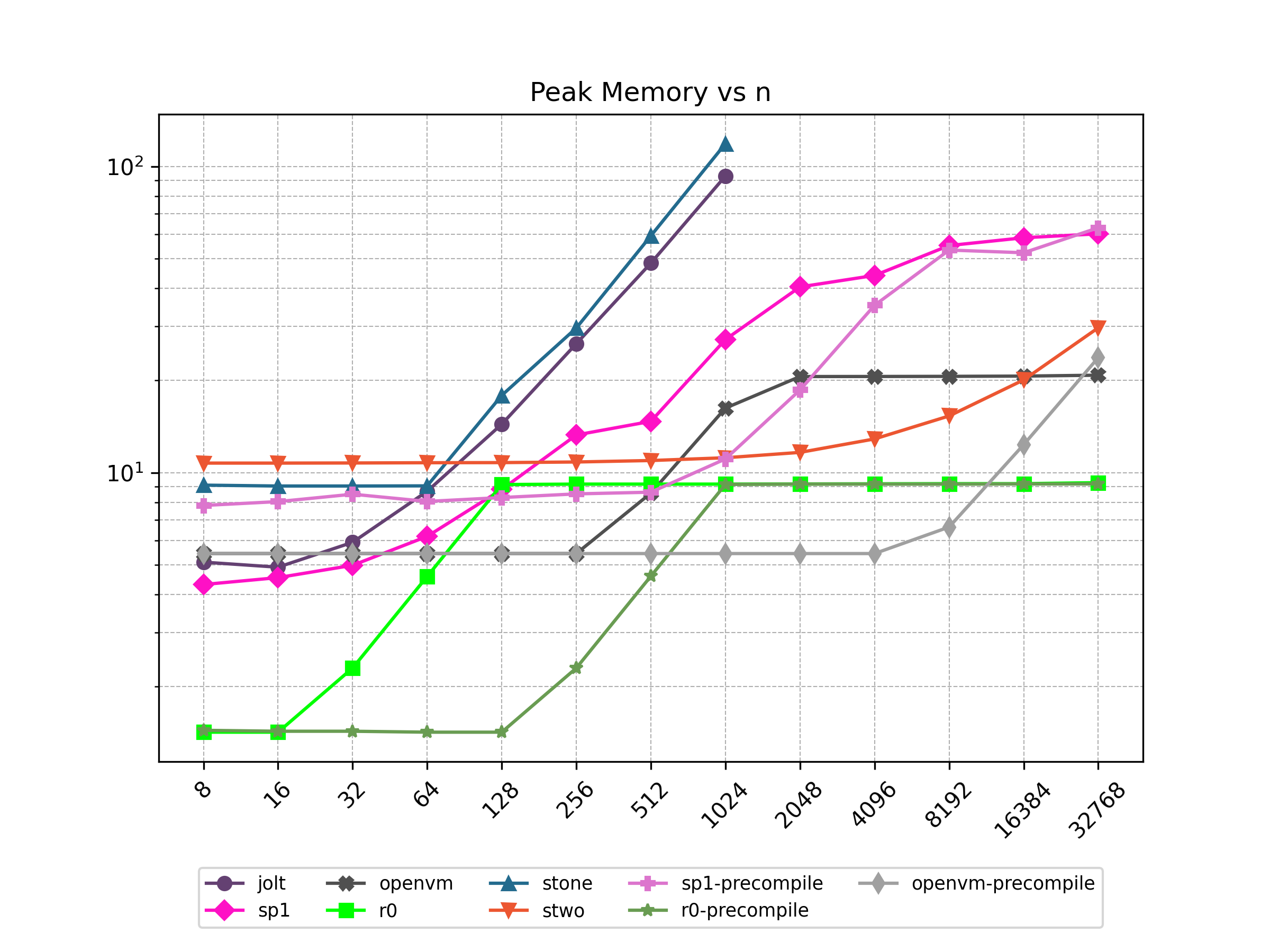
Sha3
Benchmark Keccak256 hash of n bytes. For Stone, the implementation of Keccak256 from stdlib as well as builtin was benchmarked.
Prover Time (s)
| n | jolt | sp1 | openvm | r0 | stone | stwo | sp1-precompile | r0-precompile | openvm-precompile | stone-precompile |
|---|---|---|---|---|---|---|---|---|---|---|
| 256 | 1.719 | 13.328 | 31.471 | 11.348 | 20.266 | 19.743 | 60.343 | 33.9 | 57.925 | 18.361 |
| 512 | 2.109 | 13.627 | 32.773 | 17.205 | 30.972 | 10.897 | 60.387 | 36.853 | 59.354 | 17.21 |
| 1024 | 3.15 | 15.275 | 34.777 | 17.179 | 65.925 | 23.258 | 60.193 | 42.789 | 58.748 | 18.037 |
| 2048 | 4.924 | 17.564 | 39.929 | 29.094 | 115.746 | 16.661 | 60.696 | 43.047 | 59.419 | 16.58 |
| 4096 | ❌ | 24.096 | 45.142 | 52.54 | 💾 | 11.693 | 60.073 | 54.792 | 61.503 | 27.567 |
| 8192 | ❌ | 37.851 | 60.927 | 110.08 | 💾 | 16.392 | 61.477 | 78.203 | 63.798 | 43.043 |
| 16384 | ❌ | 50.158 | 94.74 | 225.876 | 💾 | 15.422 | 63.416 | 136.103 | 70.003 | 86.217 |
| 32768 | ❌ | 66.943 | 165.212 | 422.471 | 💾 | 16.528 | 70.234 | 251.263 | 79.62 | 151.873 |
| 65536 | ❌ | 109.098 | 308.693 | 841.045 | 💾 | 21.269 | 84.047 | 437.697 | 102.599 | 💾 |
| 131072 | ❌ | 207.231 | 753.494 | 1671.26 | 💾 | 32.631 | 96.357 | 856.136 | 151.591 | 💾 |
| 262144 | ❌ | 367.867 | 1526.34 | 3310.6 | 💾 | 59.078 | 133.31 | 1691.49 | 252.934 | 💾 |
| 524288 | ❌ | 701.99 | 3048.73 | 6615.82 | 💾 | 106.153 | 191.352 | 3376.32 | 454.067 | 💾 |
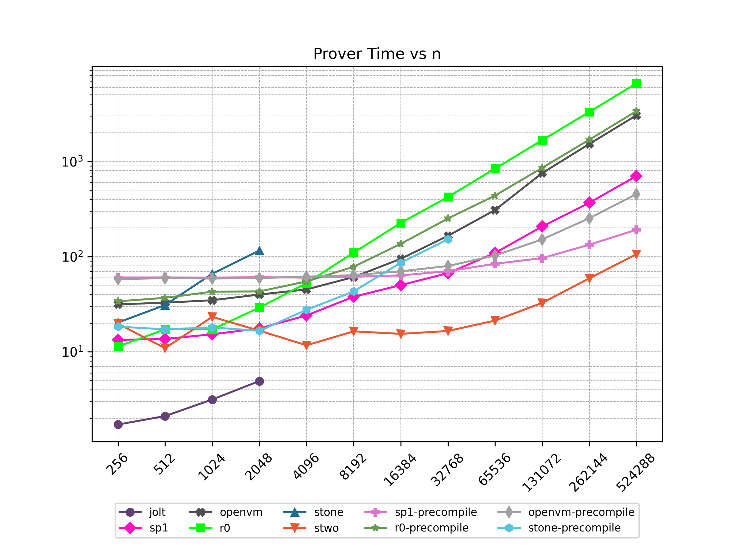
Verifier Time (ms)
| n | jolt | sp1 | openvm | r0 | stone | stwo | sp1-precompile | r0-precompile | openvm-precompile | stone-precompile |
|---|---|---|---|---|---|---|---|---|---|---|
| 256 | 77.0 | 107 | 139 | 23 | 505.0 | 11 | 116 | 24 | 141 | 269.0 |
| 512 | 66.0 | 107 | 139 | 23 | 494.0 | 11 | 108 | 23 | 141 | 213.0 |
| 1024 | 58.0 | 84 | 139 | 22 | 495.0 | 11 | 88 | 23 | 141 | 244.0 |
| 2048 | 61.0 | 109 | 140 | 24 | 544.0 | 11 | 104 | 22 | 141 | 217.0 |
| 4096 | ❌ | 110 | 140 | 22 | 💾 | 11 | 114 | 22 | 142 | 229.0 |
| 8192 | ❌ | 108 | 139 | 23 | 💾 | 11 | 89 | 22 | 142 | 254.0 |
| 16384 | ❌ | 83 | 140 | 24 | 💾 | 38 | 91 | 23 | 142 | 262.0 |
| 32768 | ❌ | 83 | 140 | 24 | 💾 | 139 | 88 | 22 | 141 | 273.0 |
| 65536 | ❌ | 82 | 140 | 24 | 💾 | 198 | 111 | 23 | 141 | 💾 |
| 131072 | ❌ | 83 | 57 | 24 | 💾 | 201 | 88 | 22 | 141 | 💾 |
| 262144 | ❌ | 83 | 56 | 23 | 💾 | 631 | 88 | 23 | 141 | 💾 |
| 524288 | ❌ | 83 | 56 | 22 | 💾 | 191 | 88 | 23 | 141 | 💾 |
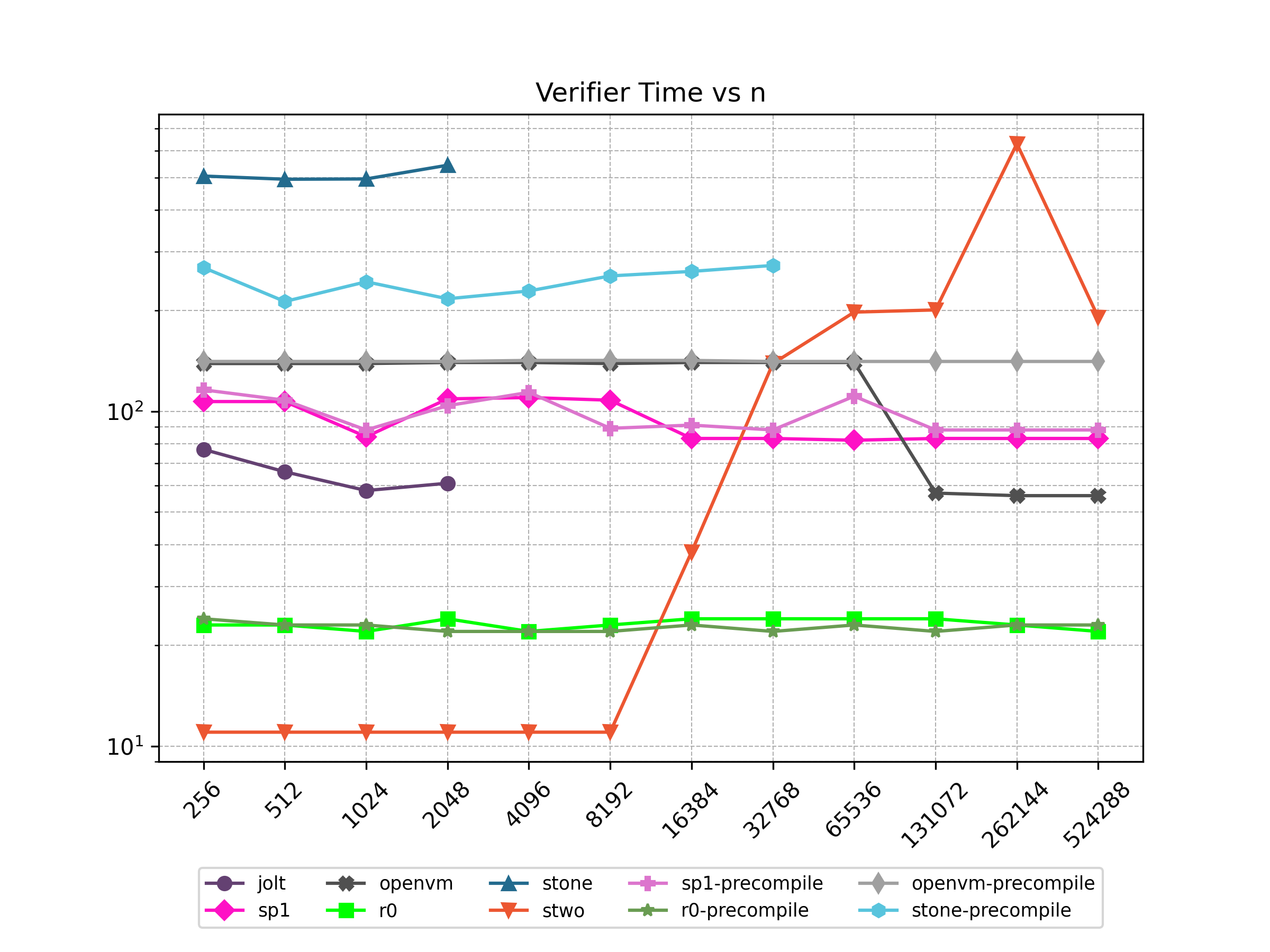
Proof Size (KB)
| n | jolt | sp1 | openvm | r0 | stone | stwo | sp1-precompile | r0-precompile | openvm-precompile | stone-precompile |
|---|---|---|---|---|---|---|---|---|---|---|
| 256 | 170.823 | 1315.56 | 1708.31 | 223.482 | 113.64 | 1002.79 | 1477.23 | 223.482 | 1787.55 | 108.008 |
| 512 | 180.175 | 1315.56 | 1708.31 | 223.482 | 119.272 | 991.494 | 1477.23 | 223.482 | 1787.55 | 107.752 |
| 1024 | 189.943 | 1315.56 | 1708.31 | 223.482 | 126.92 | 1001.15 | 1477.23 | 223.482 | 1787.55 | 110.312 |
| 2048 | 200.127 | 1315.56 | 1708.31 | 223.482 | 130.536 | 1001.4 | 1477.23 | 223.482 | 1787.55 | 110.056 |
| 4096 | ❌ | 1315.56 | 1708.31 | 223.482 | 💾 | 1016.95 | 1477.23 | 223.482 | 1787.55 | 114.92 |
| 8192 | ❌ | 1315.56 | 1708.31 | 223.482 | 💾 | 1012.45 | 1477.23 | 223.482 | 1787.55 | 119.848 |
| 16384 | ❌ | 1315.56 | 1708.31 | 223.482 | 💾 | 1027.4 | 1477.23 | 223.482 | 1787.55 | 126.088 |
| 32768 | ❌ | 1315.56 | 1708.31 | 223.482 | 💾 | 1014.61 | 1477.23 | 223.482 | 1787.55 | 132.872 |
| 65536 | ❌ | 1315.56 | 1708.31 | 223.482 | 💾 | 1037.78 | 1477.23 | 223.482 | 1787.55 | 💾 |
| 131072 | ❌ | 1315.56 | 852.937 | 223.482 | 💾 | 1073.61 | 1477.23 | 223.482 | 1787.55 | 💾 |
| 262144 | ❌ | 1315.56 | 816.649 | 223.482 | 💾 | 1154.34 | 1477.23 | 223.482 | 1787.55 | 💾 |
| 524288 | ❌ | 1315.56 | 852.937 | 223.482 | 💾 | 1179.28 | 1477.23 | 223.482 | 1787.55 | 💾 |
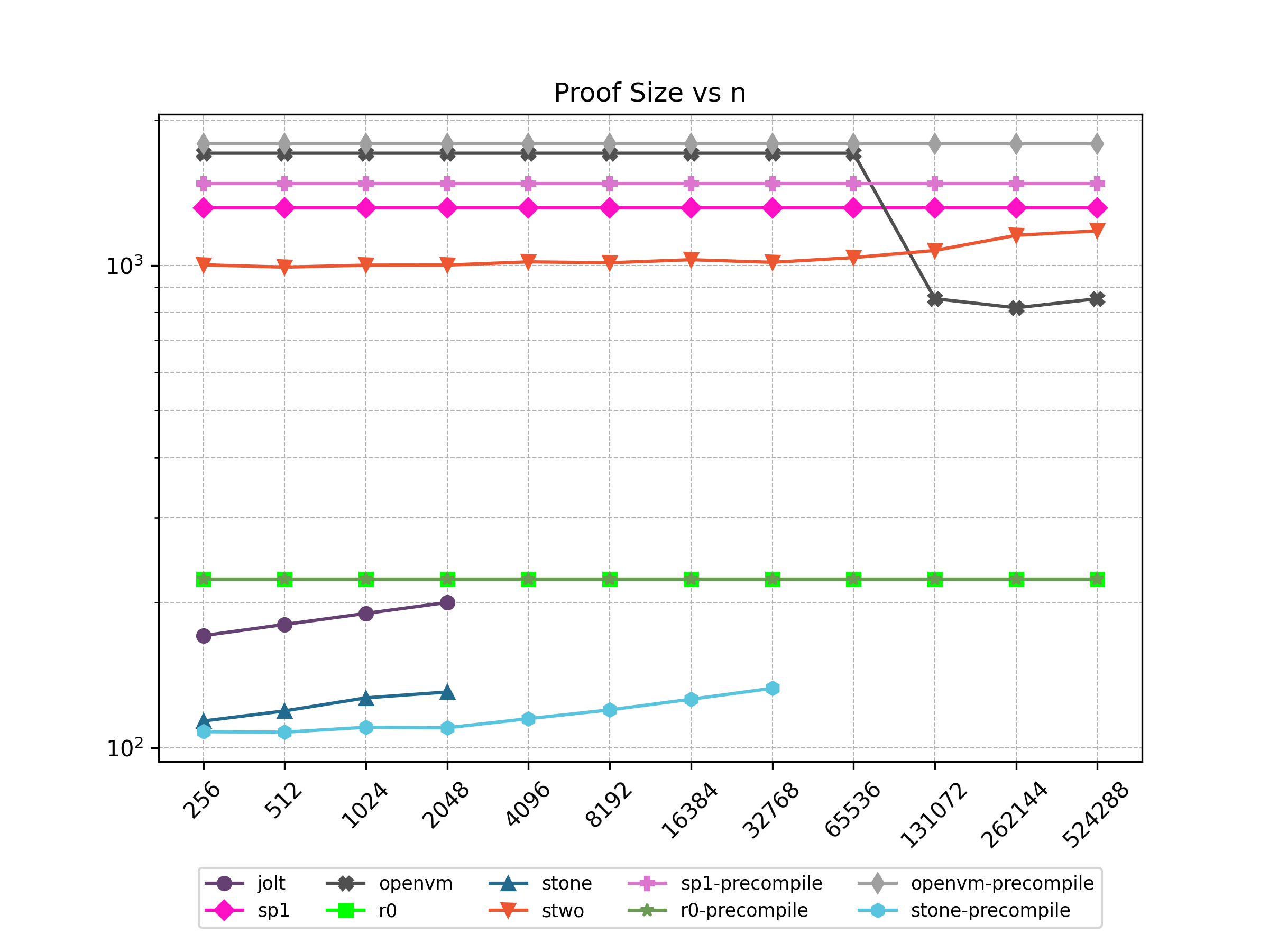
Cycle Count
| n | jolt | sp1 | r0 | stone | stwo | sp1-precompile | r0-precompile | stone-precompile |
|---|---|---|---|---|---|---|---|---|
| 256 | 46732.0 | 47653 | 63651 | 19431.0 | 131071 | 15337 | 36390 | 998.0 |
| 512 | 90274.0 | 84714 | 121925 | 38611.0 | 131071 | 20082 | 63910 | 1762.0 |
| 1024 | 177358 | 158823 | 238473 | 59058.0 | 262143 | 29559 | 118950 | 3286.0 |
| 2048 | 351574 | 307036 | 471569 | 117859 | 524287 | 48508 | 229030 | 6334.0 |
| 4096 | ❌ | 586913 | 921296 | 💾 | 1048575 | 86015 | 448102 | 12241.0 |
| 8192 | ❌ | 1146654 | 1820750 | 💾 | 2097151 | 161016 | 886246 | 24055.0 |
| 16384 | ❌ | 2266147 | 3619658 | 💾 | 2097151 | 311029 | 1762534 | 47683.0 |
| 32768 | ❌ | 4505110 | 7217474 | 💾 | 4194303 | 611032 | 3515110 | 94930.0 |
| 65536 | ❌ | 8999653 | 14429571 | 💾 | 8388607 | 1211497 | 7021350 | 💾 |
| 131072 | ❌ | 17988714 | 28853765 | 💾 | 16777215 | 2412402 | 14038604 | 💾 |
| 262144 | ❌ | 35966823 | 57702153 | 💾 | 33554431 | 4814199 | 28068169 | 💾 |
| 524288 | ❌ | 71923036 | 115398929 | 💾 | 67108863 | 9617788 | 56132428 | 💾 |
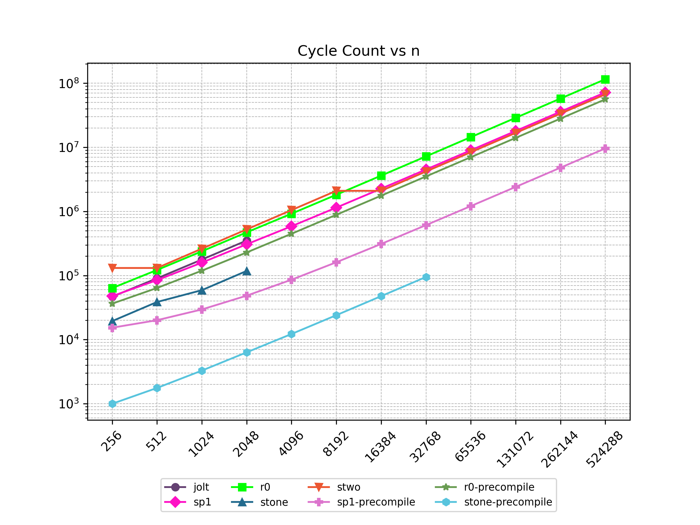
Peak Memory (GB)
| n | jolt | sp1 | openvm | r0 | stone | stwo | sp1-precompile | r0-precompile | openvm-precompile | stone-precompile |
|---|---|---|---|---|---|---|---|---|---|---|
| 256 | 5.43 | 4.5 | 5.44 | 1.42 | 19.02 | 10.82 | 11.56 | 3.46 | 5.49 | 11.13 |
| 512 | 4.9 | 4.54 | 5.44 | 2.3 | 35.74 | 10.85 | 11.59 | 3.45 | 5.49 | 11.07 |
| 1024 | 4.9 | 5.01 | 5.44 | 2.3 | 71.41 | 10.97 | 11.55 | 3.45 | 5.49 | 11.07 |
| 2048 | 5.8 | 6.16 | 5.44 | 4.59 | 142.54 | 11.21 | 11.62 | 3.45 | 5.49 | 11.07 |
| 4096 | ❌ | 8.7 | 5.44 | 9.17 | 💾 | 11.9 | 11.79 | 4.59 | 5.49 | 21.97 |
| 8192 | ❌ | 13.65 | 5.44 | 9.17 | 💾 | 13.19 | 11.96 | 9.16 | 5.49 | 43.91 |
| 16384 | ❌ | 12.24 | 5.85 | 9.18 | 💾 | 13.73 | 11.87 | 9.17 | 5.49 | 87.17 |
| 32768 | ❌ | 24.03 | 10.77 | 9.18 | 💾 | 17 | 12.23 | 9.17 | 5.48 | 174.24 |
| 65536 | ❌ | 39 | 20.53 | 9.19 | 💾 | 23.54 | 12.22 | 9.18 | 5.49 | 💾 |
| 131072 | ❌ | 52.23 | 21.23 | 9.2 | 💾 | 42.08 | 17.09 | 9.18 | 8.19 | 💾 |
| 262144 | ❌ | 52.28 | 22.77 | 9.2 | 💾 | 78.97 | 27.25 | 9.21 | 15.42 | 💾 |
| 524288 | ❌ | 57.67 | 22.93 | 9.27 | 💾 | 151.16 | 55.68 | 9.22 | 29.87 | 💾 |
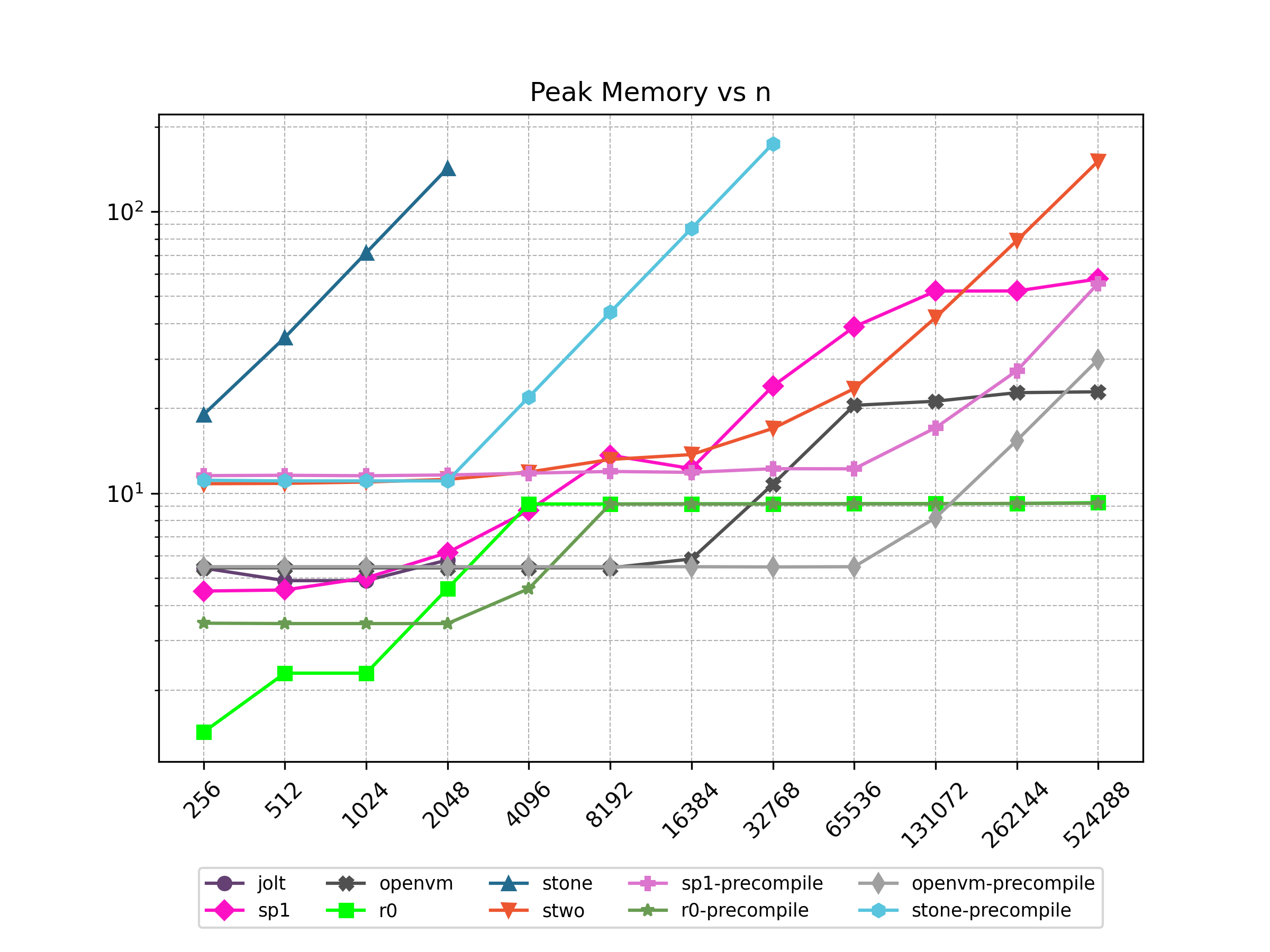
Sha3-Chain
Benchmark Keccak256 hash of 32 bytes for n iteration.
Prover Time (s)
| n | jolt | sp1 | openvm | r0 | stone | stwo | sp1-precompile | r0-precompile | openvm-precompile | stone-precompile |
|---|---|---|---|---|---|---|---|---|---|---|
| 8 | 3.151 | 14.691 | 31.427 | 17.2 | 66.291 | 13.552 | 59.266 | 34.114 | 58.806 | 16.827 |
| 16 | 5.142 | 17.431 | 34.818 | 28.941 | 115.28 | 18.47 | 60.353 | 37.322 | 59.329 | 18.279 |
| 32 | 8.57 | 23.603 | 43.135 | 52.437 | 💾 | 13.475 | 60.409 | 36.973 | 58.913 | 27.208 |
| 64 | 15.082 | 37.422 | 57.017 | 74.883 | 💾 | 14.55 | 60.377 | 42.978 | 59.971 | 43.739 |
| 128 | 29.25 | 50.151 | 90.378 | 132.931 | 💾 | 18.699 | 59.433 | 54.814 | 61.487 | 85.956 |
| 256 | 55.496 | 66.364 | 156.377 | 261.039 | 💾 | 22.329 | 61.843 | 78.503 | 65.217 | 151.067 |
| 512 | 105.689 | 104.036 | 297.659 | 515.447 | 💾 | 29.078 | 65.634 | 92.151 | 72.255 | 💾 |
| 1024 | ❌ | 192.377 | 715.326 | 1037.74 | 💾 | 52.14 | 73.4 | 176.441 | 88.201 | 💾 |
| 2048 | ❌ | 357.885 | 1474.13 | 2034.16 | 💾 | 94.358 | 91.595 | 348.058 | 115.792 | 💾 |
| 4096 | ❌ | 681.138 | 2909.76 | 4083.82 | 💾 | ❌ | 109.247 | 665.897 | 171.808 | 💾 |
| 8192 | ❌ | 1316.41 | 5795.09 | 8122.75 | 💾 | ❌ | 183.78 | 1286.1 | 510.264 | 💾 |
| 16384 | ❌ | 2597.86 | 11684.6 | 16241.2 | 💾 | ❌ | 353.935 | 2565.25 | 870.635 | 💾 |
| 32768 | ❌ | 5192.04 | 23068.5 | 32449.9 | 💾 | ❌ | 657.383 | 5090.45 | 1712.06 | 💾 |
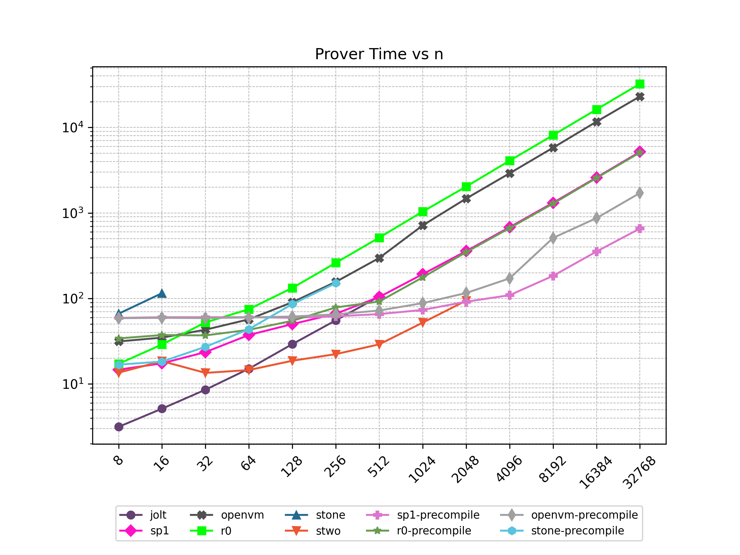
Verifier Time (ms)
| n | jolt | sp1 | openvm | r0 | stone | stwo | sp1-precompile | r0-precompile | openvm-precompile | stone-precompile |
|---|---|---|---|---|---|---|---|---|---|---|
| 8 | 83.0 | 107 | 139 | 23 | 526.0 | 11.0 | 122 | 20 | 142 | 252.0 |
| 16 | 114.0 | 86 | 139 | 23 | 555.0 | 11.0 | 116 | 23 | 142 | 254.0 |
| 32 | 75.0 | 111 | 139 | 23 | 💾 | 11.0 | 88 | 23 | 142 | 256.0 |
| 64 | 79.0 | 102 | 139 | 23 | 💾 | 11.0 | 116 | 23 | 142 | 265.0 |
| 128 | 57.0 | 99 | 139 | 23 | 💾 | 11.0 | 99 | 22 | 141 | 270.0 |
| 256 | 64.0 | 83 | 139 | 22 | 💾 | 42.0 | 90 | 20 | 141 | 288.0 |
| 512 | 118.0 | 83 | 139 | 23 | 💾 | 44.0 | 103 | 23 | 141 | 💾 |
| 1024 | ❌ | 83 | 56 | 23 | 💾 | 49.0 | 106 | 23 | 144 | 💾 |
| 2048 | ❌ | 84 | 56 | 23 | 💾 | 572.0 | 88 | 24 | 142 | 💾 |
| 4096 | ❌ | 83 | 56 | 23 | 💾 | ❌ | 88 | 23 | 141 | 💾 |
| 8192 | ❌ | 84 | 56 | 23 | 💾 | ❌ | 87 | 22 | 56 | 💾 |
| 16384 | ❌ | 83 | 55 | 20 | 💾 | ❌ | 88 | 24 | 57 | 💾 |
| 32768 | ❌ | 84 | 57 | 23 | 💾 | ❌ | 88 | 22 | 55 | 💾 |
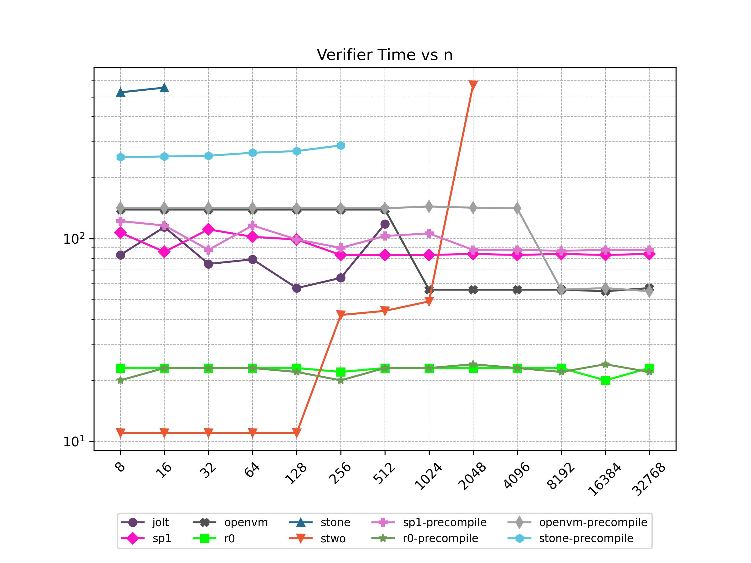
Proof Size (KB)
| n | jolt | sp1 | openvm | r0 | stone | stwo | sp1-precompile | r0-precompile | openvm-precompile | stone-precompile |
|---|---|---|---|---|---|---|---|---|---|---|
| 8 | 191.263 | 1315.56 | 1708.31 | 223.482 | 124.616 | 995.554 | 1477.23 | 223.482 | 1787.55 | 109.8 |
| 16 | 201.447 | 1315.56 | 1708.31 | 223.482 | 129.96 | 1006.302 | 1477.23 | 223.482 | 1787.55 | 108.264 |
| 32 | 212.047 | 1315.56 | 1708.31 | 223.482 | 💾 | 1028.558 | 1477.23 | 223.482 | 1787.55 | 115.944 |
| 64 | 223.063 | 1315.56 | 1708.31 | 223.482 | 💾 | 1023.458 | 1477.23 | 223.482 | 1787.55 | 122.856 |
| 128 | 234.495 | 1315.56 | 1708.31 | 223.482 | 💾 | 1032.058 | 1477.23 | 223.482 | 1787.55 | 123.304 |
| 256 | 246.343 | 1315.56 | 1708.31 | 223.482 | 💾 | 1031.81 | 1477.23 | 223.482 | 1787.55 | 131.944 |
| 512 | 258.607 | 1315.56 | 1708.31 | 223.482 | 💾 | 1084.746 | 1477.23 | 223.482 | 1787.55 | 💾 |
| 1024 | ❌ | 1315.56 | 852.937 | 223.482 | 💾 | 1155.054 | 1477.23 | 223.482 | 1787.55 | 💾 |
| 2048 | ❌ | 1315.56 | 816.649 | 223.482 | 💾 | 1182.062 | 1477.23 | 223.482 | 1787.55 | 💾 |
| 4096 | ❌ | 1315.56 | 852.937 | 223.482 | 💾 | ❌ | 1477.23 | 223.482 | 1787.55 | 💾 |
| 8192 | ❌ | 1315.56 | 816.649 | 223.482 | 💾 | ❌ | 1477.23 | 223.482 | 852.937 | 💾 |
| 16384 | ❌ | 1315.56 | 816.649 | 223.482 | 💾 | ❌ | 1477.23 | 223.482 | 852.937 | 💾 |
| 32768 | ❌ | 1315.56 | 852.937 | 223.482 | 💾 | ❌ | 1477.23 | 223.482 | 816.649 | 💾 |
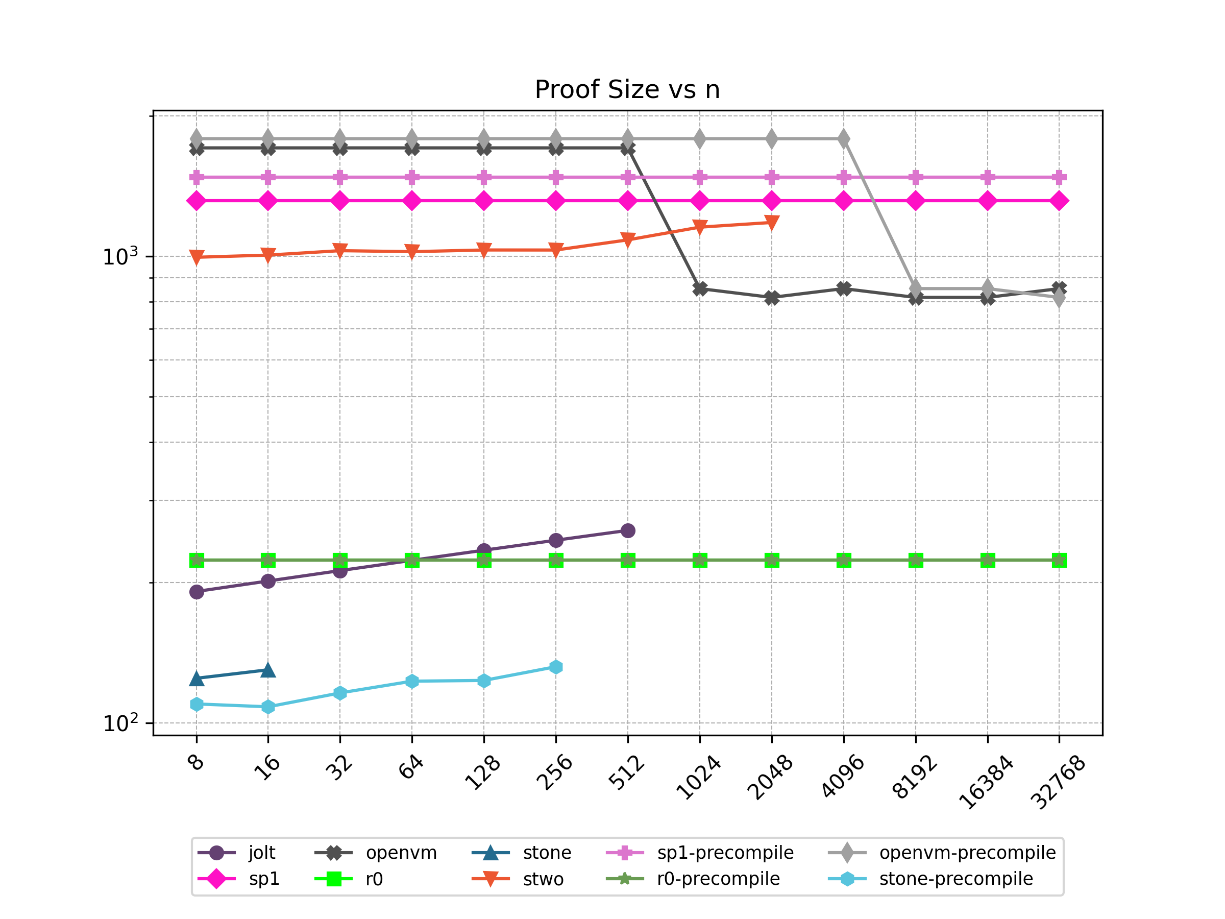
Cycle Count
| n | jolt | sp1 | r0 | stone | stwo | sp1-precompile | r0-precompile | stone-precompile |
|---|---|---|---|---|---|---|---|---|
| 8 | 203331 | 147841 | 147328 | 57648.0 | 262143 | 18577 | 27805 | 3480.0 |
| 16 | 404363 | 284353 | 286232 | 115185 | 524287 | 25825 | 43693 | 6904.0 |
| 32 | 806427 | 557377 | 564040 | 💾 | 1048575 | 40321 | 75469 | 13752.0 |
| 64 | 1610555 | 1103425 | 1119656 | 💾 | 2097151 | 69313 | 139021 | 27448.0 |
| 128 | 3218828 | 2195521 | 2230888 | 💾 | 4194303 | 127297 | 266125 | 54840.0 |
| 256 | 6435340 | 4379713 | 4453352 | 💾 | 8388607 | 243265 | 520333 | 109624 |
| 512 | 12868364 | 8748097 | 8898280 | 💾 | 16777215 | 475201 | 1028749 | 💾 |
| 1024 | ❌ | 17484865 | 17788136 | 💾 | 33554431 | 939073 | 2050355 | 💾 |
| 2048 | ❌ | 34958401 | 35567848 | 💾 | 67108863 | 1866817 | 4093575 | 💾 |
| 4096 | ❌ | 69905473 | 71127272 | 💾 | ❌ | 3722305 | 8174812 | 💾 |
| 8192 | ❌ | 139799617 | 142246120 | 💾 | ❌ | 7433281 | 16338156 | 💾 |
| 16384 | ❌ | 279587905 | 284483816 | 💾 | ❌ | 14855233 | 32669621 | 💾 |
| 32768 | ❌ | 559164481 | 568959208 | 💾 | ❌ | 29699137 | 65327886 | 💾 |
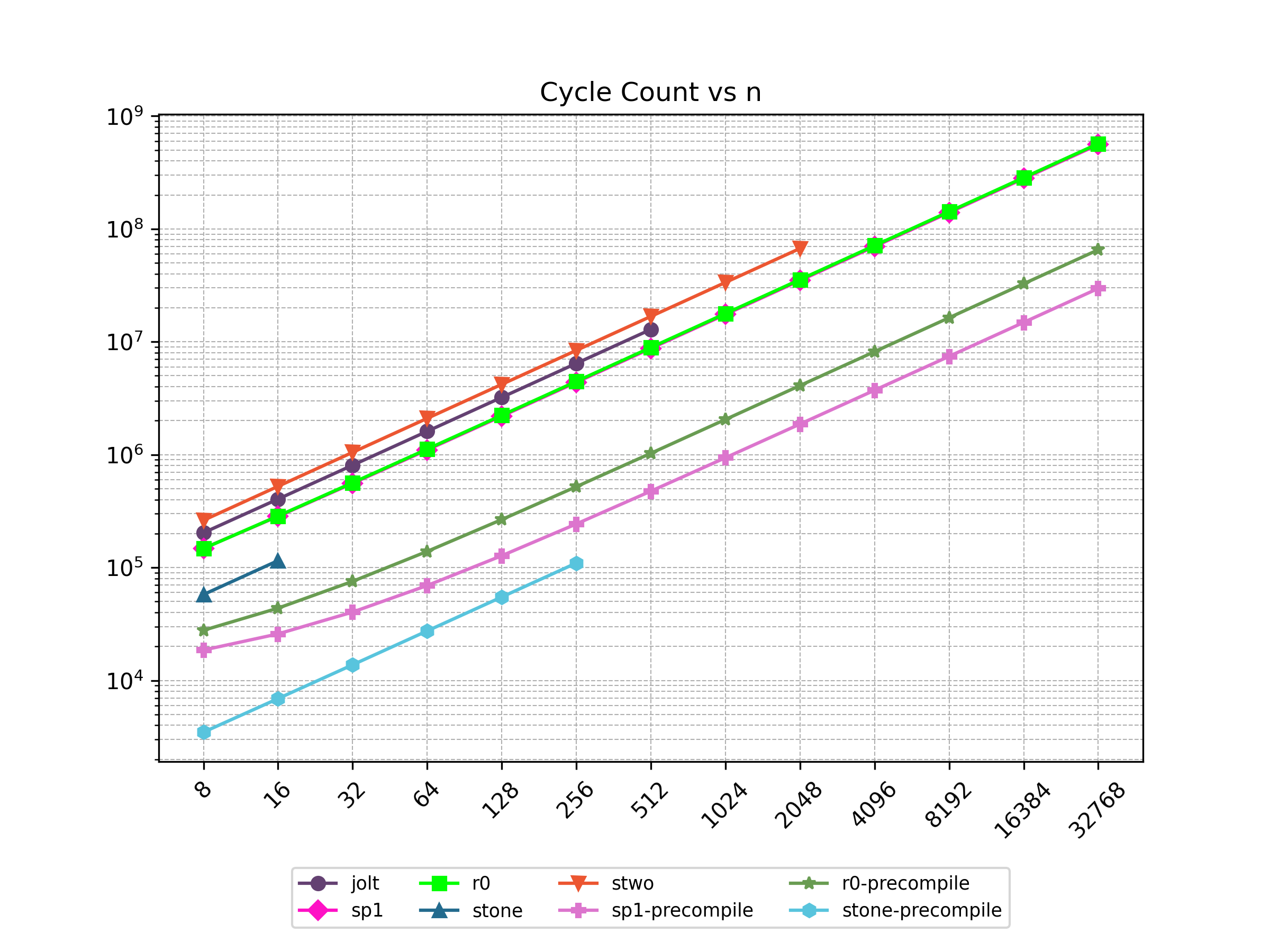
Peak Memory (GB)
| n | jolt | sp1 | openvm | r0 | stone | stwo | sp1-precompile | r0-precompile | openvm-precompile | stone-precompile |
|---|---|---|---|---|---|---|---|---|---|---|
| 8 | 5.09 | 5.14 | 5.44 | 2.3 | 71.49 | 10.95 | 11.61 | 3.45 | 5.49 | 11.07 |
| 16 | 5.85 | 6.23 | 5.44 | 4.58 | 142.53 | 11.14 | 11.43 | 3.45 | 5.49 | 11.07 |
| 32 | 8.88 | 9.03 | 5.44 | 9.14 | 💾 | 11.83 | 11.95 | 3.45 | 5.49 | 21.98 |
| 64 | 14.89 | 13.13 | 5.44 | 9.17 | 💾 | 13.2 | 11.6 | 3.45 | 5.49 | 43.91 |
| 128 | 27.13 | 12.02 | 5.7 | 9.18 | 💾 | 15.6 | 11.49 | 4.57 | 5.49 | 87.26 |
| 256 | 51.24 | 21.98 | 10.48 | 9.18 | 💾 | 20.66 | 11.14 | 9.13 | 5.49 | 174.37 |
| 512 | 100.0 | 39.84 | 19.95 | 9.18 | 💾 | 36.36 | 11.92 | 9.16 | 5.49 | 💾 |
| 1024 | ❌ | 41.18 | 19.95 | 9.19 | 💾 | 67.57 | 11.24 | 9.16 | 5.49 | 💾 |
| 2048 | ❌ | 47.4 | 19.96 | 9.2 | 💾 | 128.39 | 14.17 | 9.16 | 6.28 | 💾 |
| 4096 | ❌ | 59.51 | 20.31 | 9.22 | 💾 | ❌ | 30.3 | 9.17 | 11.39 | 💾 |
| 8192 | ❌ | 61.16 | 20.5 | 9.26 | 💾 | ❌ | 53.85 | 9.18 | 20.72 | 💾 |
| 16384 | ❌ | 61.43 | 20.75 | 9.34 | 💾 | ❌ | 57.23 | 9.2 | 20.8 | 💾 |
| 32768 | ❌ | 63.58 | 20.93 | 9.49 | 💾 | ❌ | 63.67 | 9.22 | 20.87 | 💾 |
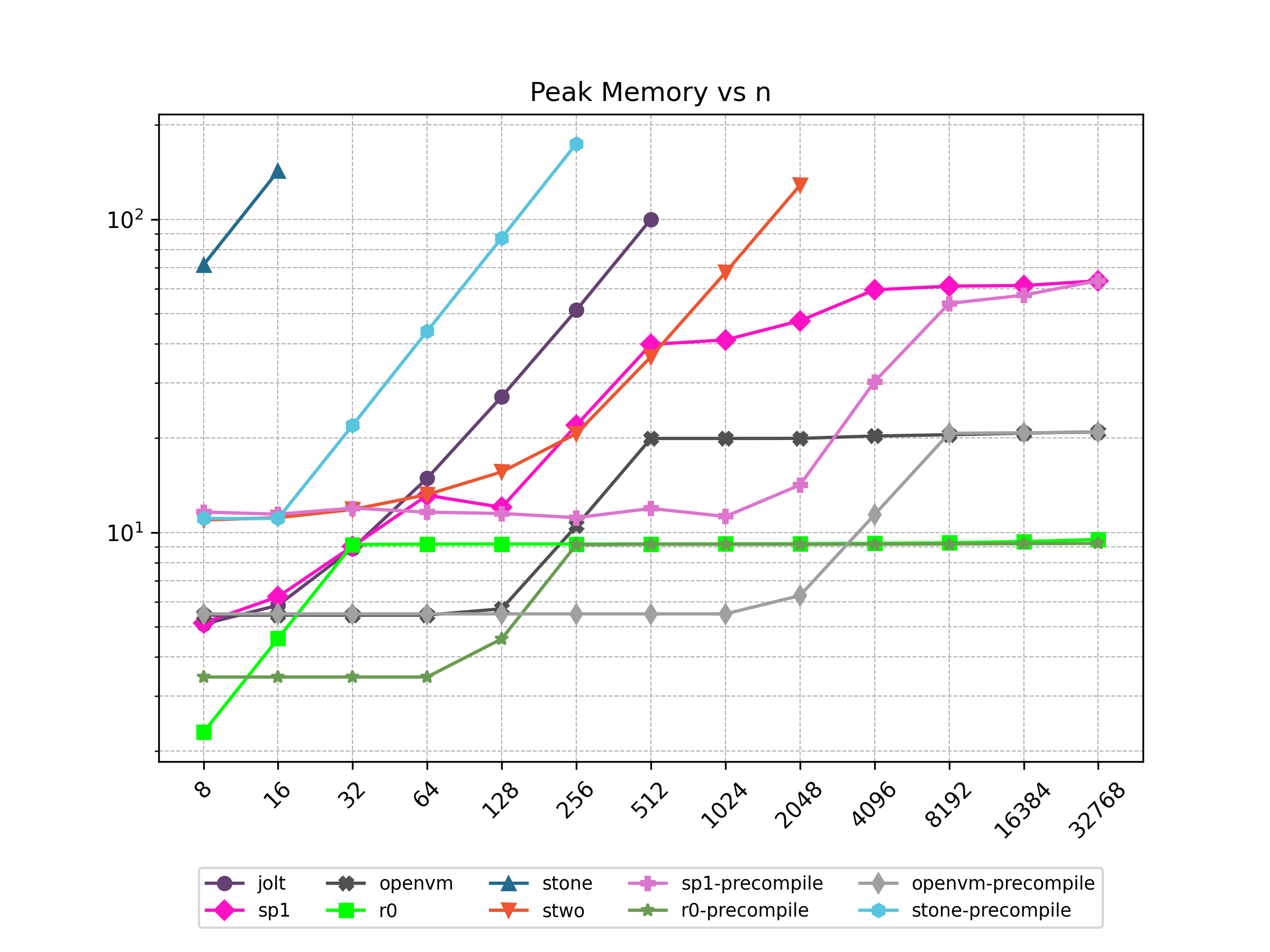
BLAKE
Benchmark Blake2s256 hash of n bytes. For the Stwo benchmarks, a dedicated opcode for BLAKE was used, as illustrated in this Cairo source file. SP1 and R0 do not support precompiles for BLAKE.
Prover Time (s)
| n | sp1 | r0 | stwo-precompile |
|---|---|---|---|
| 2048 | 14.272 | 28.817 | 35.206 |
| 4096 | 14.773 | 52.33 | 34.752 |
| 8192 | 17.678 | 65.67 | 30.911 |
| 16384 | 24.308 | 126.219 | 32.214 |
| 32768 | 37.485 | 240.843 | 30.324 |
| 65536 | 55.119 | 476.273 | 38.614 |
| 131072 | 101.786 | 947.306 | 35.269 |
| 262144 | 162.863 | 1888.15 | 33.434 |
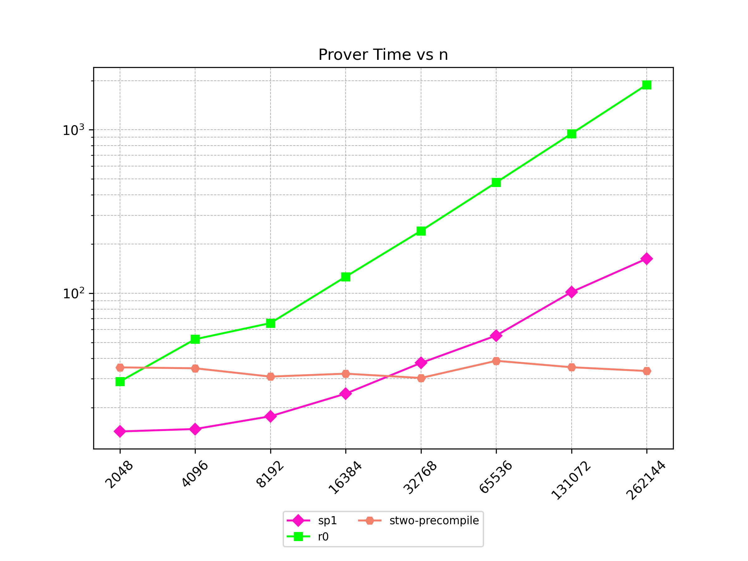
Verifier Time (ms)
| n | sp1 | r0 | stwo-precompile |
|---|---|---|---|
| 2048 | 102 | 10 | 11 |
| 4096 | 105 | 23 | 11 |
| 8192 | 111 | 22 | 11 |
| 16384 | 99 | 24 | 11 |
| 32768 | 104 | 23 | 12 |
| 65536 | 81 | 22 | 12 |
| 131072 | 81 | 23 | 37 |
| 262144 | 81 | 22 | 48 |
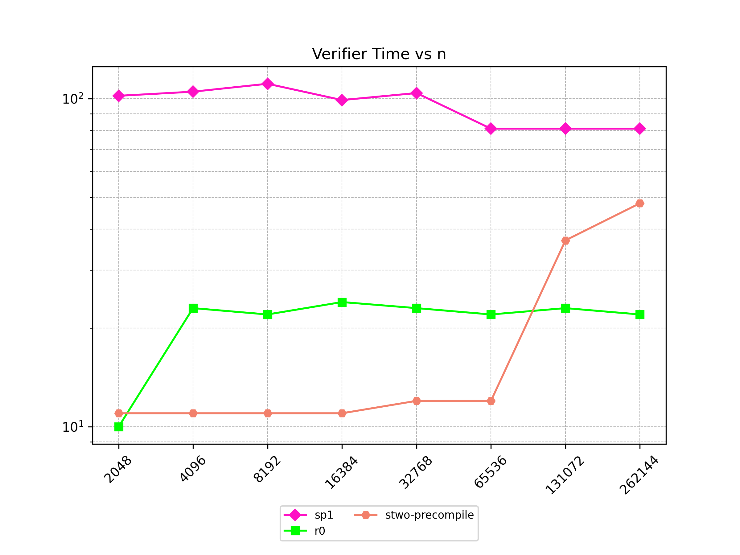
Proof Size (KB)
| n | sp1 | r0 | stwo-precompile |
|---|---|---|---|
| 2048 | 1315.56 | 223.482 | 1117.14 |
| 4096 | 1315.56 | 223.482 | 1138.83 |
| 8192 | 1315.56 | 223.482 | 1134.37 |
| 16384 | 1315.56 | 223.482 | 1121.81 |
| 32768 | 1315.56 | 223.482 | 1144.87 |
| 65536 | 1315.56 | 223.482 | 1158.19 |
| 131072 | 1315.56 | 223.482 | 1141.67 |
| 262144 | 1315.56 | 223.482 | 1148.66 |
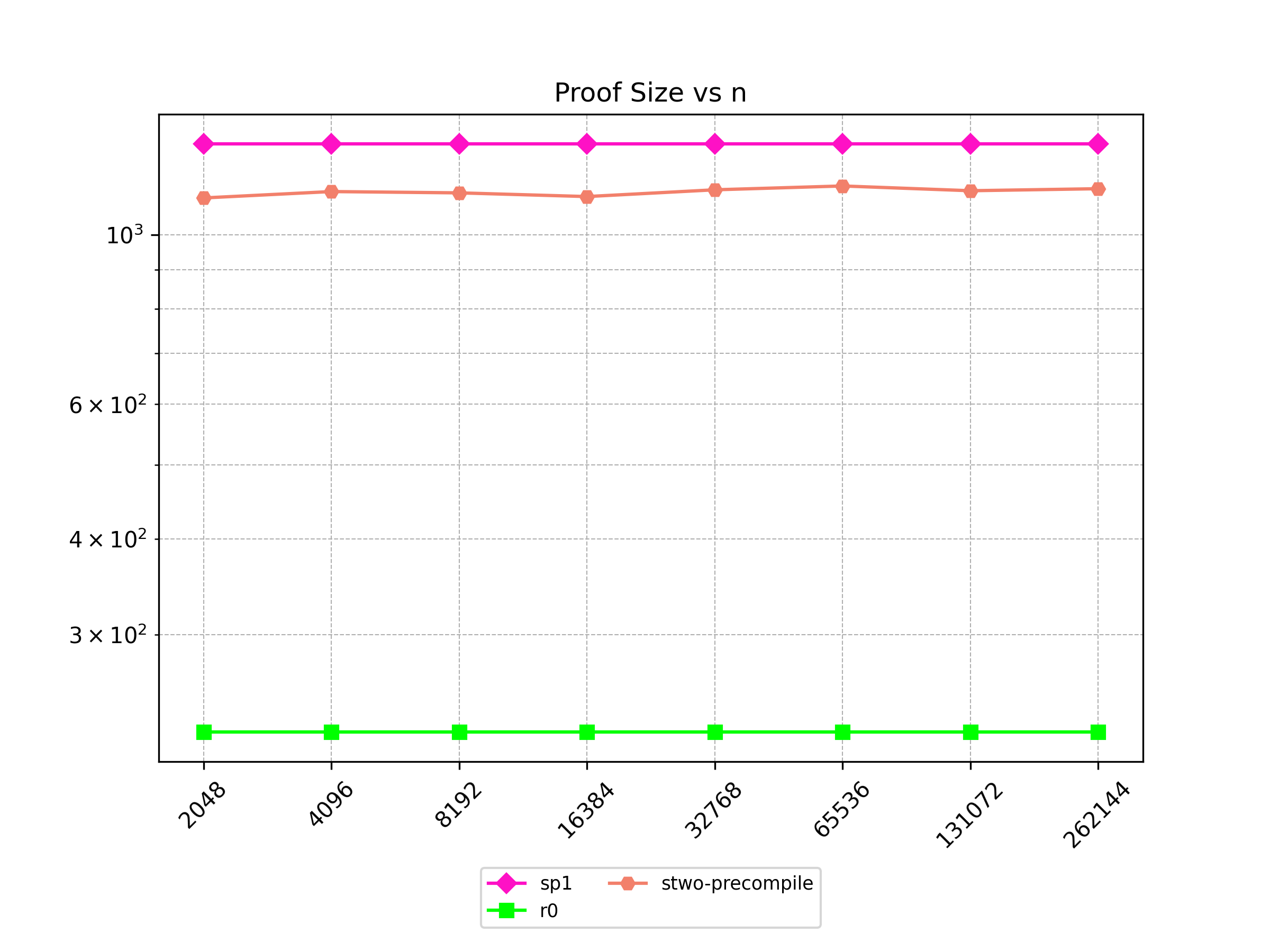
Cycle Count
| n | sp1 | r0 | stwo-precompile |
|---|---|---|---|
| 2048 | 100997 | 264515 | 65535 |
| 4096 | 193061 | 521763 | 65535 |
| 8192 | 377189 | 1036259 | 65535 |
| 16384 | 745445 | 2065251 | 65535 |
| 32768 | 1481957 | 4123235 | 131071 |
| 65536 | 2954981 | 8239203 | 262143 |
| 131072 | 5901029 | 16471139 | 524287 |
| 262144 | 11793125 | 32935011 | 1048575 |
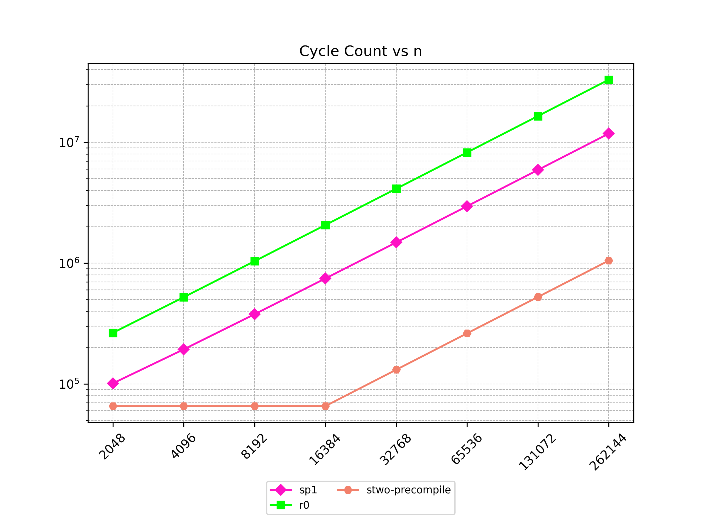
Peak Memory (GB)
| n | sp1 | r0 | stwo-precompile |
|---|---|---|---|
| 2048 | 4.55 | 4.58 | 19.98 |
| 4096 | 5 | 9.14 | 19.94 |
| 8192 | 6.09 | 9.17 | 19.98 |
| 16384 | 8.83 | 9.18 | 20.02 |
| 32768 | 13.83 | 9.18 | 20.17 |
| 65536 | 16.59 | 9.18 | 20.5 |
| 131072 | 38 | 9.19 | 20.88 |
| 262144 | 45.31 | 9.19 | 21.97 |
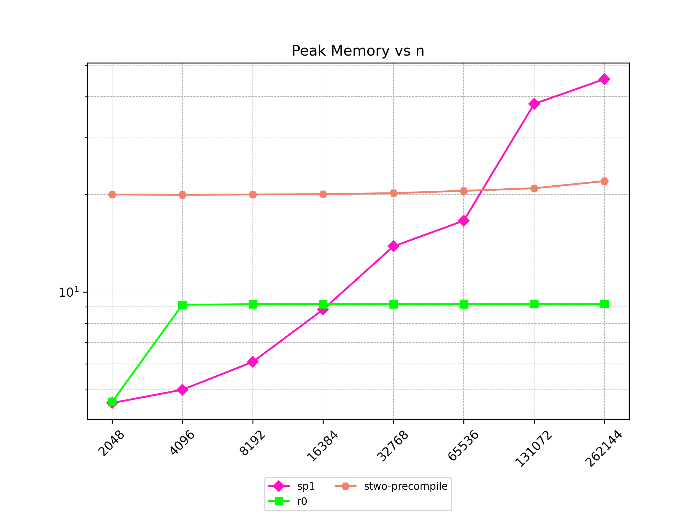
BLAKE-Chain
Benchmark Blake2s256 hash of 32 bytes for n iteration. For the Stwo benchmarks, a dedicated opcode for BLAKE was used, as illustrated in this Cairo source file. SP1 and R0 do not support precompiles for BLAKE.
Prover Time (s)
| n | sp1 | r0 | stwo-precompile |
|---|---|---|---|
| 128 | 17.319 | 28.76 | 30.885 |
| 256 | 24.279 | 52.074 | 32.974 |
| 512 | 38.5 | 86.181 | 33.26 |
| 1024 | 53.129 | 166.706 | 30.723 |
| 2048 | 89.423 | 316.029 | 38.153 |
| 4096 | 145.299 | 628.118 | 31.717 |
| 8192 | 259.23 | 1260.14 | 37.422 |
| 16384 | 495.878 | 2521.17 | 35.82 |
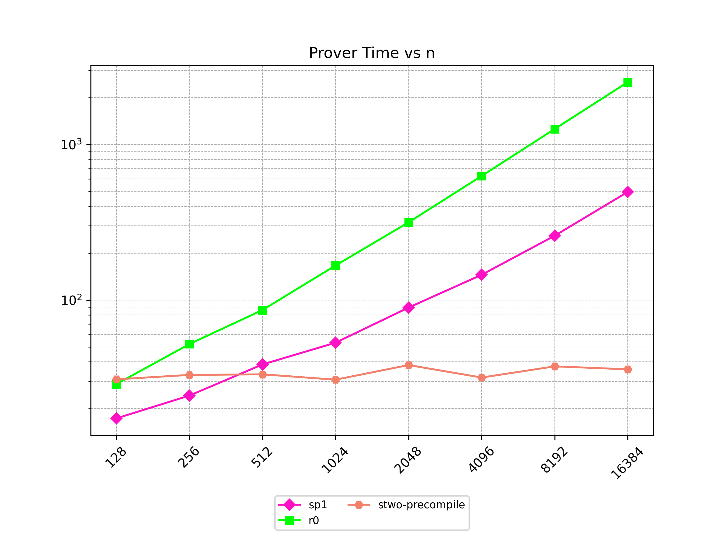
Verifier Time (ms)
| n | sp1 | r0 | stwo-precompile |
|---|---|---|---|
| 128 | 105 | 22 | 11 |
| 256 | 104 | 22 | 11 |
| 512 | 108 | 23 | 11 |
| 1024 | 84 | 23 | 11 |
| 2048 | 81 | 23 | 41 |
| 4096 | 85 | 23 | 40 |
| 8192 | 81 | 23 | 49 |
| 16384 | 81 | 22 | 39 |

Proof Size (KB)
| n | sp1 | r0 | stwo-precompile |
|---|---|---|---|
| 128 | 1315.56 | 223.482 | 1119.07 |
| 256 | 1315.56 | 223.482 | 1121.09 |
| 512 | 1315.56 | 223.482 | 1128.54 |
| 1024 | 1315.56 | 223.482 | 1119.77 |
| 2048 | 1315.56 | 223.482 | 1127.81 |
| 4096 | 1315.56 | 223.482 | 1127.26 |
| 8192 | 1315.56 | 223.482 | 1134 |
| 16384 | 1315.56 | 223.482 | 1143.83 |
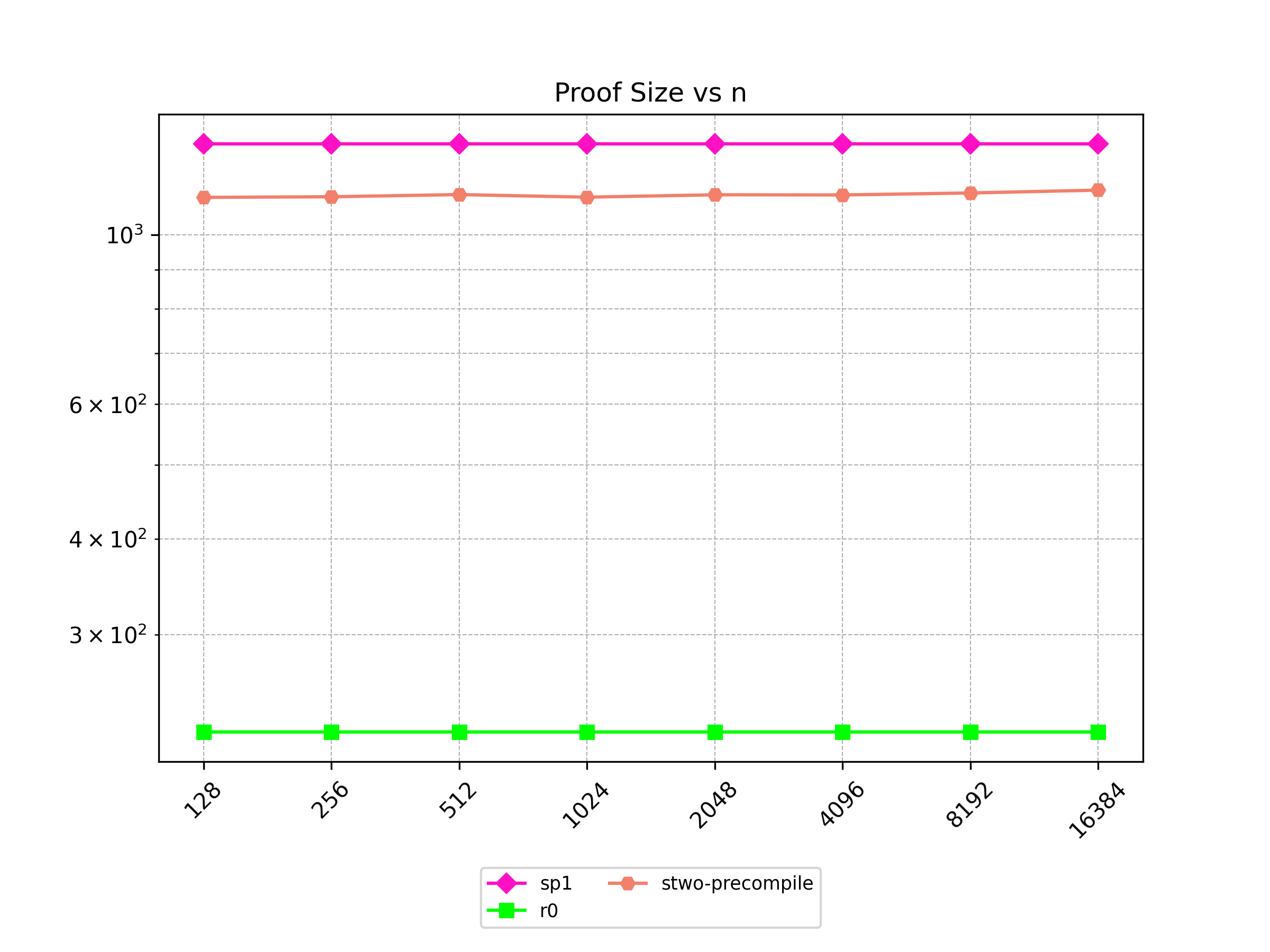
Cycle Count
| n | sp1 | r0 | stwo-precompile |
|---|---|---|---|
| 128 | 376249 | 356507 | 65535 |
| 256 | 742841 | 702491 | 65535 |
| 512 | 1476025 | 1394459 | 131071 |
| 1024 | 2942393 | 2778395 | 262143 |
| 2048 | 5875129 | 5546267 | 524287 |
| 4096 | 11740601 | 11082011 | 1048575 |
| 8192 | 23471545 | 22153499 | 2097151 |
| 16384 | 46933433 | 44296475 | 4194303 |
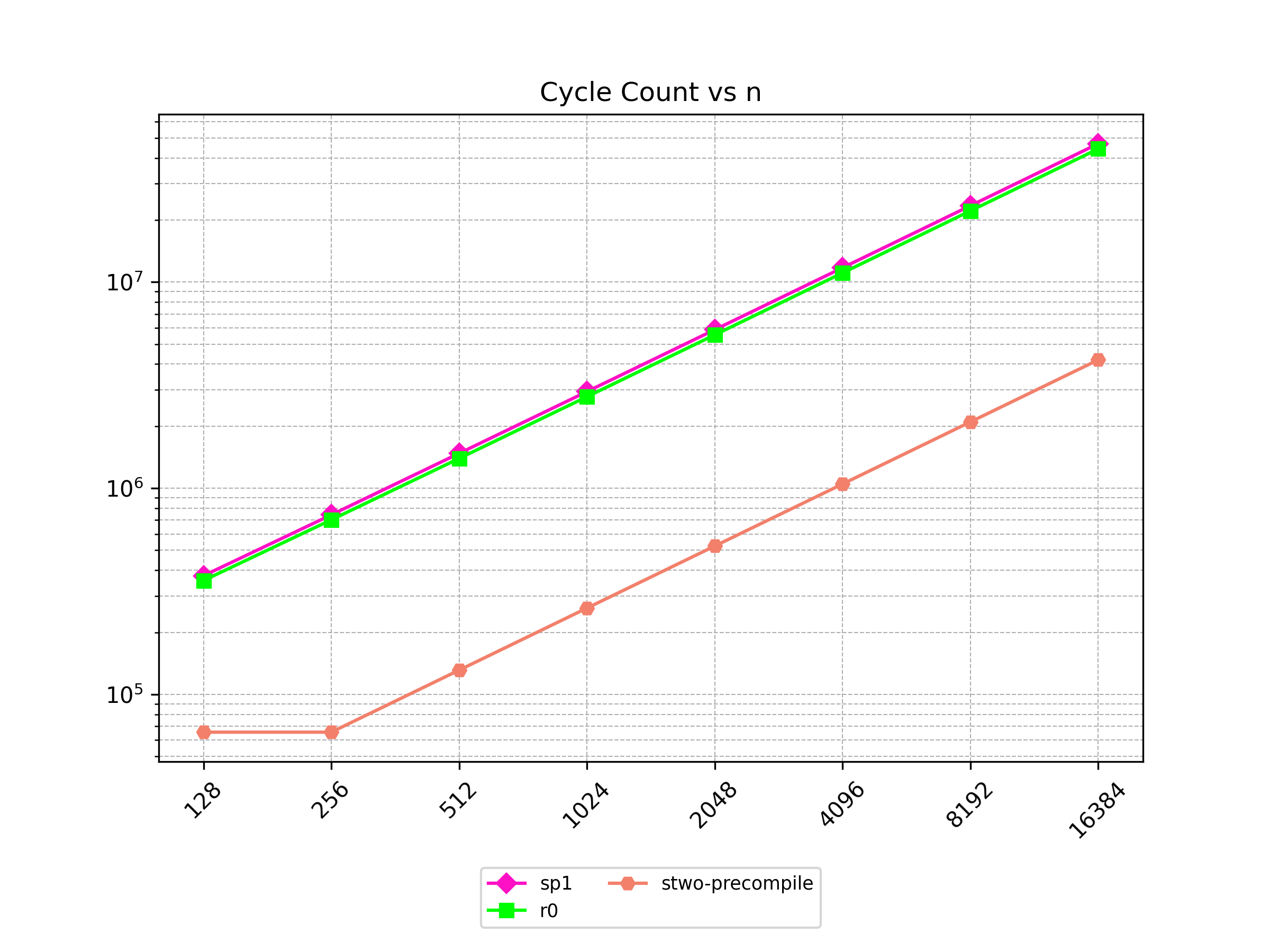
Peak Memory (GB)
| n | sp1 | r0 | stwo-precompile |
|---|---|---|---|
| 128 | 6.16 | 4.58 | 19.99 |
| 256 | 9.12 | 9.15 | 20.01 |
| 512 | 13.17 | 9.17 | 20.13 |
| 1024 | 15.96 | 9.17 | 20.39 |
| 2048 | 32.88 | 9.17 | 20.72 |
| 4096 | 44.6 | 9.19 | 21.54 |
| 8192 | 50.57 | 9.19 | 23.31 |
| 16384 | 53.25 | 9.21 | 27.19 |
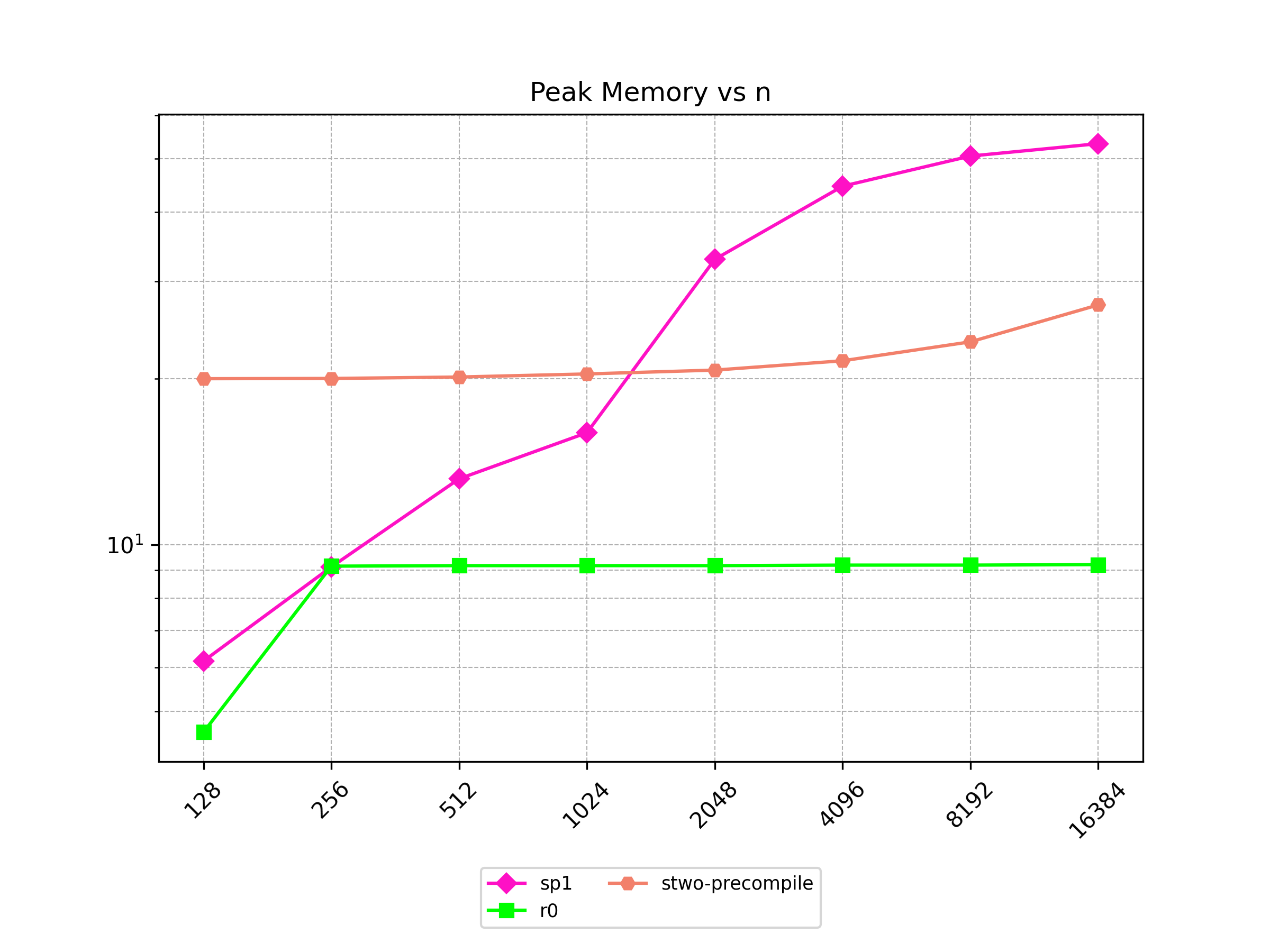
Matrix Multiplication
Benchmark multiplication of two matrices of size n x n.
Prover Time (s)
| n | jolt | sp1 | openvm | r0 | stone | stwo |
|---|---|---|---|---|---|---|
| 4 | 1.196 | 13.179 | 29.508 | 6.763 | 10.922 | 12.72 |
| 8 | 1.648 | 12.862 | 30.119 | 8.21 | 9.879 | 19.566 |
| 16 | 4.979 | 15.252 | 33.467 | 17.135 | 26.384 | 16.531 |
| 32 | 27.702 | 26.491 | 58.102 | 65.806 | 💾 | 14.655 |
| 64 | ❌ | 135.352 | 292.125 | 480.724 | 💾 | 21.199 |
| 128 | ❌ | 881.29 | 2671.68 | 3809.76 | 💾 | 76.061 |
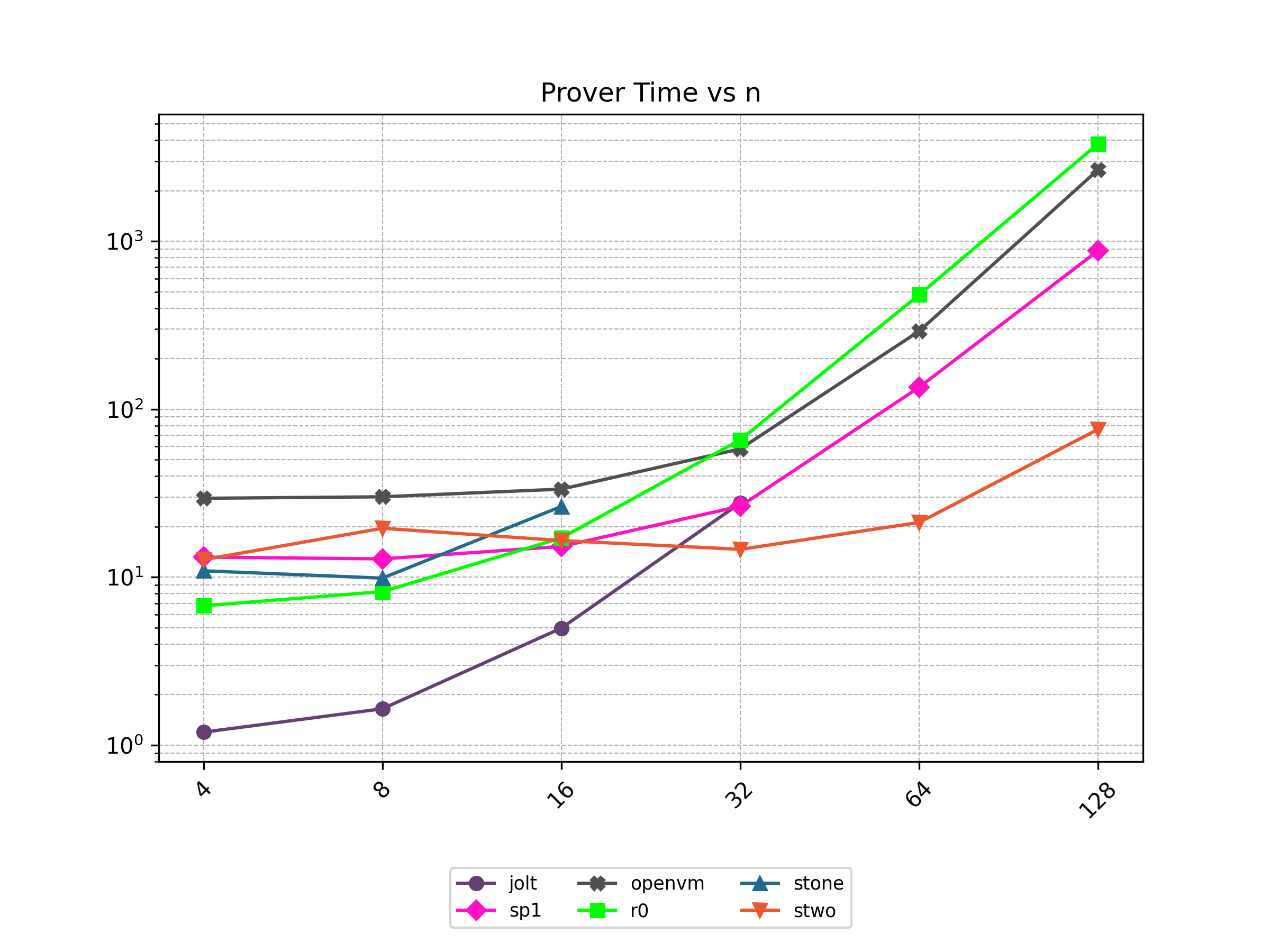
Verifier Time (ms)
| n | jolt | sp1 | openvm | r0 | stone | stwo |
|---|---|---|---|---|---|---|
| 4 | 44.0 | 110 | 140 | 23 | 111.0 | 10 |
| 8 | 51.0 | 110 | 140 | 22 | 120.0 | 10 |
| 16 | 86.0 | 102 | 139 | 23 | 139.0 | 10 |
| 32 | 84.0 | 109 | 140 | 25 | 💾 | 18 |
| 64 | ❌ | 85 | 140 | 22 | 💾 | 41 |
| 128 | ❌ | 84 | 56 | 23 | 💾 | 45 |
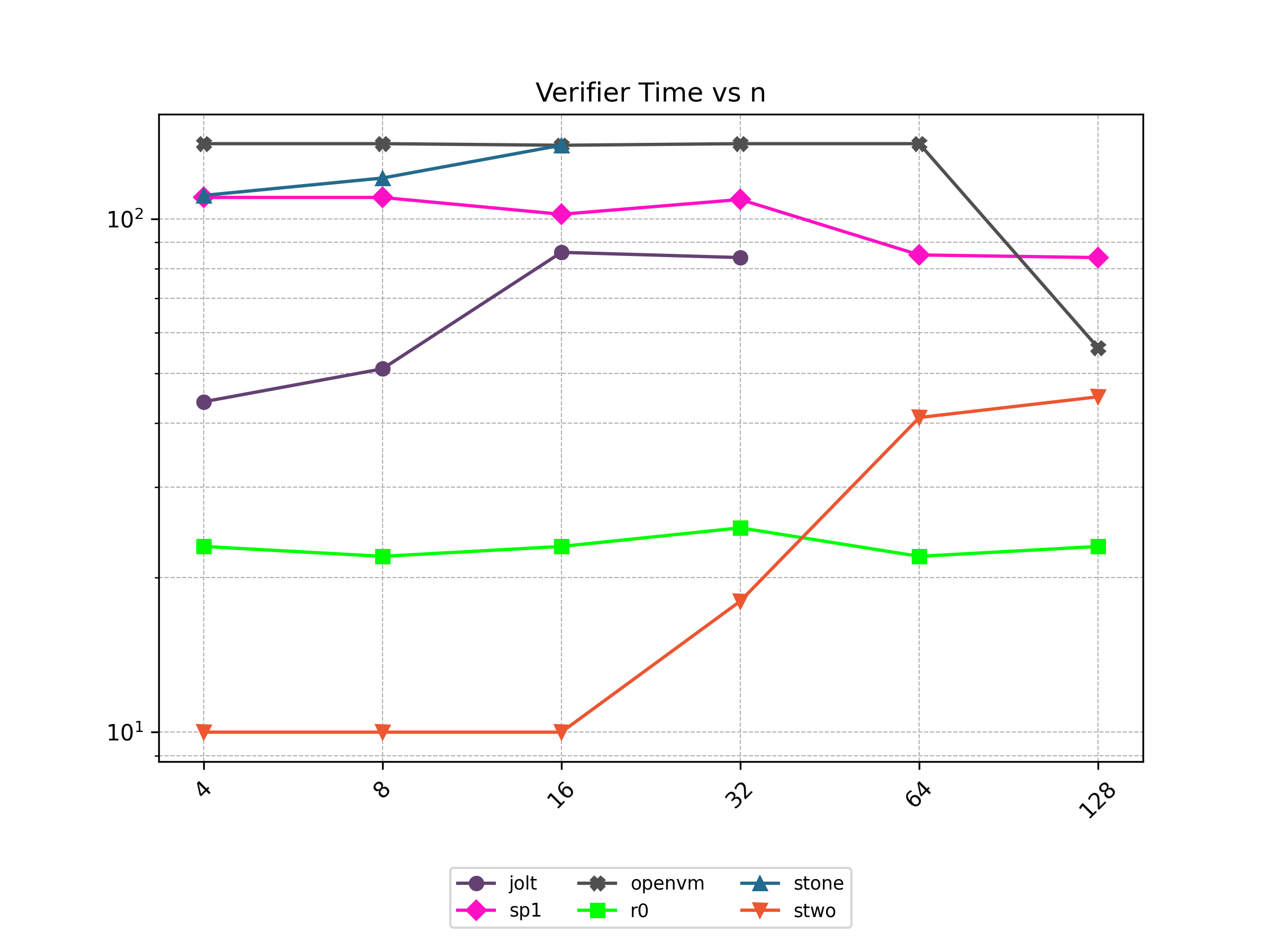
Proof Size (KB)
| n | jolt | sp1 | openvm | r0 | stone | stwo |
|---|---|---|---|---|---|---|
| 4 | 144.647 | 1315.53 | 1708.31 | 223.234 | 109.032 | 815.674 |
| 8 | 169.607 | 1315.53 | 1708.31 | 223.234 | 108.52 | 833.086 |
| 16 | 198.911 | 1315.53 | 1708.31 | 223.234 | 116.456 | 844.238 |
| 32 | 233.591 | 1315.53 | 1708.31 | 223.234 | 💾 | 844.914 |
| 64 | ❌ | 1315.53 | 1708.31 | 223.234 | 💾 | 876.354 |
| 128 | ❌ | 1315.53 | 852.937 | 223.234 | 💾 | 981.178 |
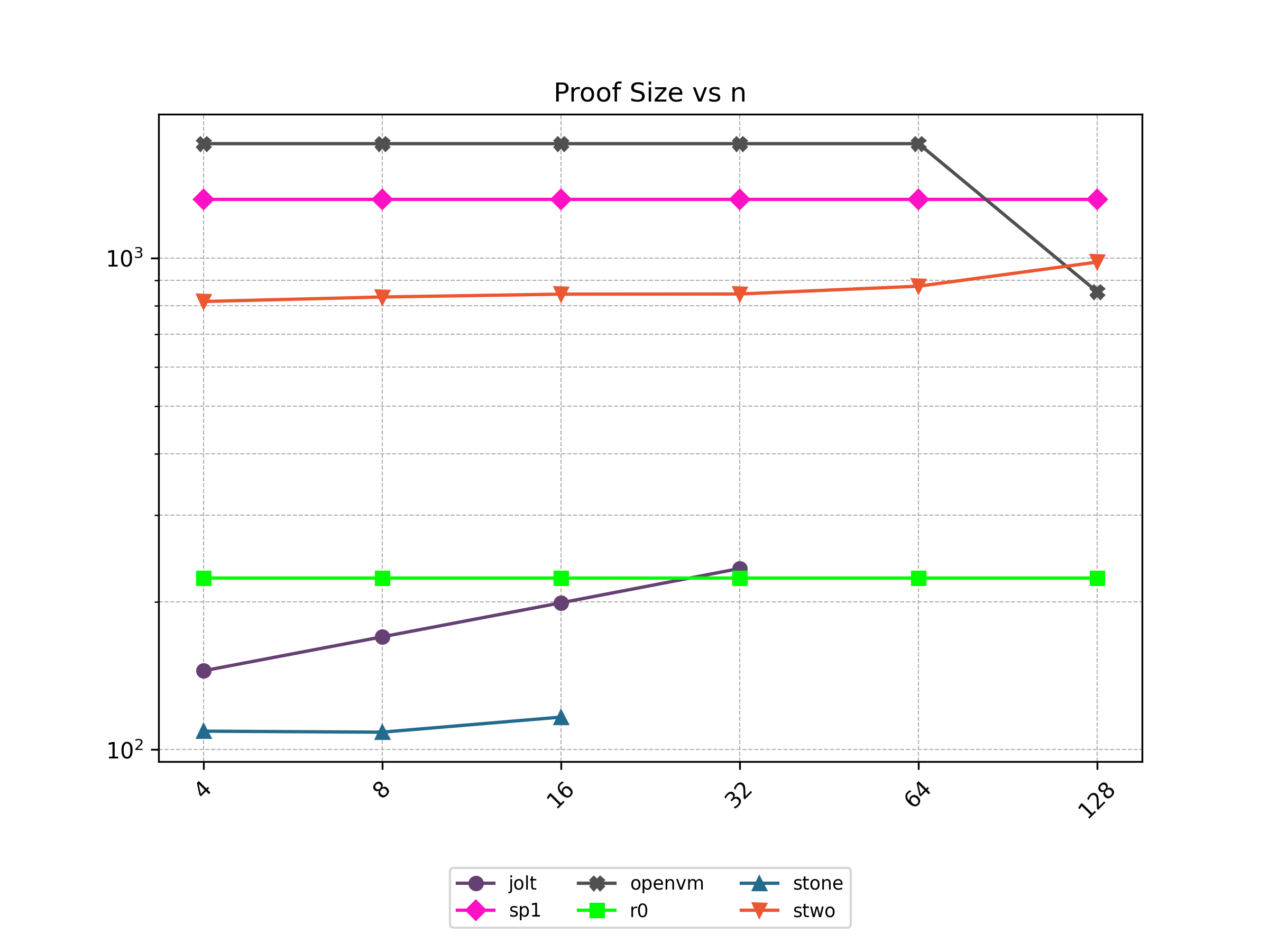
Cycle Count
| n | jolt | sp1 | r0 | stone | stwo |
|---|---|---|---|---|---|
| 4 | 7181.0 | 8430 | 5820 | 2181.0 | 32767 |
| 8 | 42753.0 | 23951 | 21352 | 13521.0 | 32767 |
| 16 | 314782 | 139844 | 137280 | 94569.0 | 131071 |
| 32 | 2457710 | 1044394 | 1041904 | 💾 | 1048575 |
| 64 | ❌ | 8211062 | 8208720 | 💾 | 8388607 |
| 128 | ❌ | 65306638 | 65304592 | 💾 | 67108863 |
Peak Memory (GB)
| n | jolt | sp1 | openvm | r0 | stone | stwo |
|---|---|---|---|---|---|---|
| 4 | 5.43 | 4.45 | 5.43 | 1.42 | 9.09 | 10.73 |
| 8 | 4.91 | 4.29 | 5.43 | 1.43 | 9.03 | 10.73 |
| 16 | 5.8 | 5.12 | 5.43 | 2.29 | 29.68 | 10.82 |
| 32 | 26.45 | 10.34 | 5.43 | 9.17 | 💾 | 11.61 |
| 64 | ❌ | 39.28 | 19.69 | 9.17 | 💾 | 19.92 |
| 128 | ❌ | 60.01 | 20.09 | 9.19 | 💾 | 101.6 |
Elliptic Curve Addition
Benchmark n point doubling for secp256k1.
Prover Time (s)
| n | jolt | sp1 | openvm | r0 | stone | stwo |
|---|---|---|---|---|---|---|
| 256 | 50.41 | 70.731 | 158.631 | 283.941 | 18.869 | 11.993 |
| 512 | 96.814 | 116.11 | 292.691 | 531.309 | 30.529 | 19.268 |
| 1024 | ❌ | 211.962 | 582.356 | 1037.16 | 65.693 | 15.356 |
| 2048 | ❌ | 394.022 | 1048.01 | 2072.757 | 114.312 | 14.318 |
| 4096 | ❌ | 741.169 | 2029.72 | 4079.796 | 💾 | 14.407 |
| 8192 | ❌ | 1426.64 | 4046.32 | 8181.789 | 💾 | 16.635 |
| 16384 | ❌ | 2844.32 | 7953.88 | ❌ | 💾 | 24.382 |
| 32768 | ❌ | 5628.39 | 15793.7 | ❌ | 💾 | 28.304 |
Verifier Time (ms)
| n | jolt | sp1 | openvm | r0 | stone | stwo |
|---|---|---|---|---|---|---|
| 256 | 67.0 | 83 | 140 | 22.0 | 188.0 | 10 |
| 512 | 60.0 | 83 | 140 | 23.0 | 181.0 | 10 |
| 1024 | ❌ | 83 | 56 | 23.0 | 187.0 | 34 |
| 2048 | ❌ | 83 | 56 | 25.0 | 238.0 | 39 |
| 4096 | ❌ | 83 | 57 | 23.0 | 💾 | 41 |
| 8192 | ❌ | 83 | 56 | 11.0 | 💾 | 36 |
| 16384 | ❌ | 83 | 56 | ❌ | 💾 | 130 |
| 32768 | ❌ | 83 | 55 | ❌ | 💾 | 15 |
Proof Size (KB)
| n | jolt | sp1 | openvm | r0 | stone | stwo |
|---|---|---|---|---|---|---|
| 256 | 249.399 | 1315.56 | 1708.31 | 223.482 | 111.592 | 918.41 |
| 512 | 261.663 | 1315.56 | 1708.31 | 223.482 | 120.04 | 897.182 |
| 1024 | ❌ | 1315.56 | 852.937 | 223.482 | 127.784 | 889.49 |
| 2048 | ❌ | 1315.56 | 852.937 | 223.482 | 131.976 | 896.15 |
| 4096 | ❌ | 1315.56 | 816.649 | 223.482 | 💾 | 901.758 |
| 8192 | ❌ | 1315.56 | 816.649 | 223.482 | 💾 | 910.154 |
| 16384 | ❌ | 1315.56 | 852.937 | ❌ | 💾 | 929.282 |
| 32768 | ❌ | 1315.56 | 816.649 | ❌ | 💾 | 931.042 |
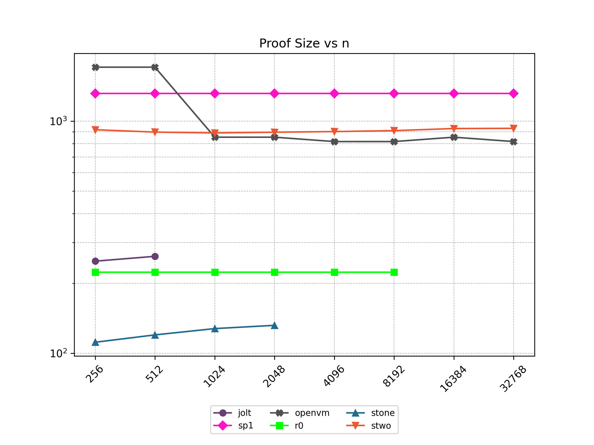
Cycle Count
| n | jolt | sp1 | r0 | stone | stwo |
|---|---|---|---|---|---|
| 256 | 4760760 | 4715656 | 4711913 | 59936.0 | 131071 |
| 512 | 9290168 | 9169544 | 9165801 | 119840 | 262143 |
| 1024 | ❌ | 18077320 | 18073577 | 239648 | 262143 |
| 2048 | ❌ | 35892872 | 35889129 | 479264 | 524287 |
| 4096 | ❌ | 71523976 | 71520233 | 💾 | 1048575 |
| 8192 | ❌ | 142786184 | 142782441 | 💾 | 2097151 |
| 16384 | ❌ | 285310600 | ❌ | 💾 | 4194303 |
| 32768 | ❌ | 570359432 | ❌ | 💾 | 8388607 |
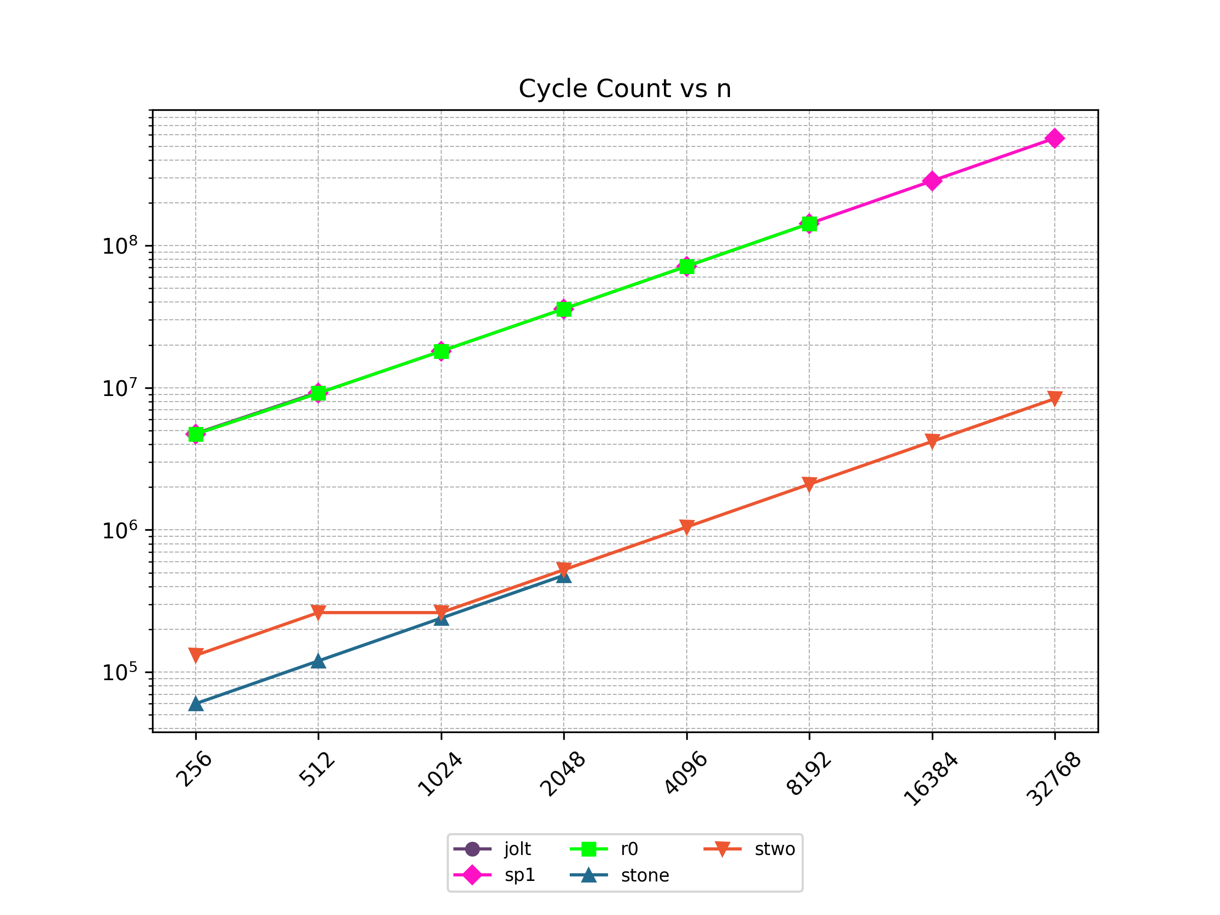
Peak Memory (GB)
| n | jolt | sp1 | openvm | r0 | stone | stwo |
|---|---|---|---|---|---|---|
| 256 | 48.62 | 23.6 | 10.37 | 9.18 | 17.93 | 10.9 |
| 512 | 93.9 | 47.38 | 19.8 | 9.19 | 35.7 | 11.08 |
| 1024 | ❌ | 44.31 | 19.83 | 9.19 | 71.47 | 11.27 |
| 2048 | ❌ | 55.82 | 19.84 | 9.19 | 142.68 | 11.81 |
| 4096 | ❌ | 62.49 | 19.86 | 9.22 | 💾 | 13.22 |
| 8192 | ❌ | 63.14 | 19.94 | 9.26 | 💾 | 16.01 |
| 16384 | ❌ | 66.48 | 19.95 | ❌ | 💾 | 21.62 |
| 32768 | ❌ | 66.97 | 19.96 | ❌ | 💾 | 32.64 |